2.1 Introduction
No doubt you have encountered linear equations many times during your careers as students. Most likely, the very first equation you had to solve was linear. Yet despite their simplicity, systems of linear equations are of immense importance in mathematics and its applications to areas of physical sciences, economics, engineering and many many more. One of the purposes of linear algebra is to undertake a systematic study of linear equations. In this lab, we will use MATLAB to solve systems of linear equations. We will also learn about a very useful application of systems of linear equations to economics and computer science.
2.2 Systems of Linear Equations
By now we have seen how a system of linear equations can be transformed into a matrix equation, making the system easier to solve. For example, the system
can be written the following way:

Now, by augmenting the matrix with the vector on the right and using row operations, this equation can easily be solved by hand. However, if our system did not have nice integer entries, solving the system by hand using row reduction could become very difficult. MATLAB provides us with an easier way to get an answer.
A system of this type has the form Ax = b, so we can enter these numbers into MATLAB using the following commands:
>> A = [2 -1 1; 1 2 3; 3 0 -1]
>> b = [8; 9; 3]
(Notice that for the column vector b, we include semicolons after each entry to ensure that the entries are on different rows; the command
>> b = [8 9 3]
would produce a row vector, which is not the same thing.)
The command
>> x = A\b
will find the solution (if it exists) to our equation Ax = b. In this case, MATLAB tells us
x
=
2.0000
-1.0000
3.0000
Remark 2.1 Please take care in entering "A\b" command. It has a backslash "\" and NOT a forward slash "/".
| Exercise 2.1 | |
| (a) Consider the system
of equations: 2x1 + x2 + 5x3 = -1 x1 + 6x3 = 2 -6x1 + 2x2 + 4x3 = 3 On paper, convert this system of equations into a matrix equation of the form Cx = d. |
|
| (b) Enter the matrix C and
the column vector d into
MATLAB, and use the command
>> x = C\d to check your solution. |
|
| (c) We would expect to
get the column vector d in
MATLAB if we ran the command C*x,
right? In other words, C*x - d should
be zero. Enter this equation into MATLAB:
>> C*x-d What do you get? |
|
Remark 2.2 The discrepancy in part (c) of the above exercise is simply due to rounding error. You'll notice that the error is a vector multiplied by a very small number, one on the order of 10-15. But why is there any error at all? After all, solving by row reduction gave very nice numbers, right? The reason lies in the way MATLAB stores numbers. In this calculation MATLAB represents numbers in "floating point form", which means it represents them in scientifc notation to 10^(-14) accuracy. Thus when you see 10^(-14) printed in calculations, it is equivalent to zero.
There is a drawback, however, to solving systems of equations using the command "x = C\d". Let us explore that further.
| Exercise 2.2 Consider
the following system of equations:
-10x1 +
4x2 =
0 >> x = C\d Note the strange output. Include it in your write up. Now go ahead and solve this system by hand. How many free variables do you need to write down the solution? Based on your answer, can you explain why you got the error message when trying to use "x = C\d" command? |
To deal with the case of inconsistent systems or systems with infinitely many solutions, it may sometimes be better to use MATLAB to simply row-reduce your matrix and then read off the solutions. We happen to be very lucky since MATLAB has a command that performs Gaussian elimination for you.
Consider the following homogeneous system of equations:
6x1 +
2x2 + 3x3 =
0
4x1 + x2 -
2x3 = 0
2x1 + x2 +
5x3 = 0
Enter the corresponding matrix C and the column vector d into MATLAB. Now we want to perform row reduction on the augmented matrix [C| d]. The command that performs row reduction in MATLAB is called "rref" (it stands for "reduced row echelon form"). Then type in
>> rref([C
d])
ans
=
1.0000 0
-3.5000 0
0
1.0000
12.0000 0
0
0
0 0
Recall
from class that we can then use the row reduced form to get that
x1 = 3.5x3
x2 =-12x3
x3 here is the free variable, and it can be chosen
to be any value. Once chosen, the two equations above determine
the values of x1 and x2.
For instance, if we choose x3 = 2, then x1
= 7 and x2 = -24. In
this way we can write down all the solutions (of which there are
infinitely many) to the system above.
| Exercise 2.3 | |
| (a) Consider the
following homogeneous system of equations:
x1 -
3x2 +
2x3 =
0 |
|
2.3 An Application to Economics: Leontief Models
Wassily Leontief (1906-1999) was a Russian-born, American economist who, aside from developing highly sophisticated economic theories, also enjoyed trout fishing, ballet and fine wines. He won the 1973 Nobel Prize in economics for his work in creating mathematical models to describe various economic phenomena. In the remainder of this lab we will look at a very simple special case of his work called a closed exchange model. Here is the premise:
Suppose in a far away land of Eigenbazistan, in a small country town called Matrixville, there lived a Farmer, a Tailor, a Carpenter, a Coal Miner and Slacker Bob. The Farmer produced food; the Tailor, clothes; the Carpenter, housing; the Coal Miner supplied energy; and Slacker Bob made High Quality 100 Proof Moonshine, half of which he drank himself. Let us make the following assumptions:
Everyone buys from and sells to the central pool (i.e. there is no outside supply and demand)
Everything produced is consumed
For these reasons this is called a closed exchange model. Next we must specify what fraction of each of the goods is consumed by each person in our town. Here is a table containing this information:
| Food | Clothes | Housing | Energy | High Quality 100 Proof Moonshine | |
| Farmer | 0.25 | 0.15 | 0.25 | 0.18 | 0.20 |
| Tailor | 0.15 | 0.28 | 0.18 | 0.17 | 0.05 |
| Carpenter | 0.22 | 0.19 | 0.22 | 0.22 | 0.10 |
| Coal Miner | 0.20 | 0.15 | 0.20 | 0.28 | 0.15 |
| Slacker Bob | 0.18 | 0.23 | 0.15 | 0.15 | 0.50 |
So for example, the Carpenter consumes 22% of all food, 19% of all clothes, 22% of all housing, 22% of all energy and 10% of all High Quality 100 Proof Moonshine.
| Exercise 2.4 Note that the columns in this table all add up to 1. Explain why this happens. |
Now, let pF, pT, pC, pCM, pSB denote the incomes of the Farmer, Tailor, Carpenter, Coal Miner and Slacker Bob, respectively. Note that each of these quantities not only denotes the incomes of each of our esteemed citizens, but also the cost of the corresponding goods. So for example,pF is the Farmer's income as well as the cost of all the food. So if the Farmer produces $100 worth of food, then his income will also be $100 since all of this food is bought out and the profits go to the Farmer.
The idea is, of course, to be able to figure out how should we price the goods in order for the citizens of Matrixville to survive; i.e. we must find pF, pT, pC, pCM, and pSB subject to the following conditions:
0.25pF +
0.15pT +
0.25pC +
0.18pCM +
0.20pSB = pF
0.15pF +
0.28pT +
0.18pC +
0.17pCM +
0.05pSB = pT
0.22pF +
0.19pT +
0.22pC +
0.22pCM +
0.10pSB = pC
0.20pF +
0.15pT +
0.20pC +
0.28pCM +
0.15pSB = pCM
0.18pF +
0.23pT +
0.15pC +
0.15pCM +
0.50pSB = pSB
| Exercise 2.5 Explain where this system of equations came from and what it means. (Think about what the left hand side and the right hand side of each equation mean.) |
Let us denote the column vector (pF, pT, pC, pCM , pSB)T by p, and let C be the coefficient matrix of the above system. We can now rewrite that system as
Cp = p
or equivalently
Cp - p = Cp - Ip = (C - I)p = 0
where I is the 5x5 matrix with 1's on the diagonal and 0's everywhere else. The property of the matrix I we are using is that Iv = v for any vector v.
| Exercise 2.6 | |
| (a) Enter the matrices C and I into
MATLAB.
>> C
= [0.25 0.15 0.25 0.18 0.20; >> I = eye(5) Note that the command "eye(n)" creates an n x n matrix with 1's on the diagonal and 0's elsewhere. |
|
| (b) Use MATLAB to row reduce the augmented matrix [C - I | 0] and write down the general solution to (C - I)p = 0. | |
| (c) What are the highest and the lowest priced commodities in Matrixville? List the inhabitants of this charming town in order of increasing income. If our friend Bob makes $40,000 per year, what are the incomes for the rest of the inhabitants? With all the moonshine that Bob drinks, do you think he will live long enough to enjoy his good life? | |
2.4 How Google Works
The beginning of this story is actually a theorem of Perron-Frobenius from the early 20th century, but we will discuss this later in our tale. Instead we start with a cute word problem illustrating the theorem, which has amused linear algebra students at least as far back as the 1970's. The problem is: In a particular group of people, who is the most popular?
One possible approach is to ask everyone in the group to list their friends in that group. Say there are 4 people, named Jane, Charlie, Mary and Fred, who we affectionately nickname J, C, M and F. The friends list is:
Jane
lists C and M
Charlie lists J, M and F
Mary lists J, C and F
Fred lists J and M
(This experiment is dangerous. You should not try it in your own dormitory.) Our data naturally amounts to a 4x4 matrix of 0's and 1's:
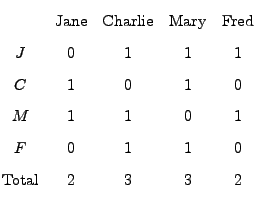
Some people tend to list every one they ever met and others only list closest friends, so to compensate for this we normalize the matrix by dividing each list by the number of people in it:
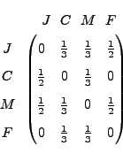
We
shall call this the linking
matrix and denote it
by L
Now that we have collected data, we wish to determine a
nonnegative number associated to each person called their popularity;
combined they give the popularity
vector 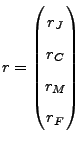 for
the group. Its basic property is
for
the group. Its basic property is
A person's popularity is the weighted sum of the popularity of people who reference that person.
We see what the weights are and what this means by the example,
which seems reasonable when one considers that Charlie's contribution to Jane's popularity is (1/3)rCharlie, because Jane constitutes one third of Charlie's friends and rCharlie is Charlie's popularity. In matrix vector form these equations are exactly
Lr = r (Equation A.1)
which is the same as
(L - I)r = 0
where I is the 4x4 identity matrix. Solving this equation we can determine the relative "popularity" of Jane, Charlie, Mary an Fred. We ran MATLAB using the rref command as in exercise 2.6 and set (arbitrarily, of course) rF = 1 to get rJ = 1.5, rC = 1.3125, rM = 1.6875, and rF = 1. Thus the order of popularity, from highest to lowest, is: Mary, Jane, Charlie, and finally, Fred.
Some graduate students at Stanford got the idea that this sort of method could be used to rank a group of web pages. You type in some key words (which we will denote by the set K) and the software identifies vast numbers of webpages WK (most of which are garbage as far as you are concerned) containing the words in K. The big challenge is automatically finding a few good (popular) webpages. What the Google founders did was have the software look at each webpage w in WK and determine which other web pages in WK the page w links to, thus associating to each webpage w a vector Lw of 0's and 1's, just as we did above with the list of students. Next, it builds a matrix L whose columns are the normalized vectors Lw and proceeds just as we did in the popularity problem. Google computes r very quickly and lists for you, the user, the web pages in order of high to low popularity.
Sounds like a good plan, but if you are going to base a company on this
and put up lots of money to back it, there are few things you would
definitely want to know:
(a) Does the equation Lr = r above
always have a solution (what do you know from the course so far makes you
think it seldom will?)
(b) Will a solution have entries that are nonnegative?
(c) Is the solution unique? If not, we will have
conflicting rankings.
Fortunately, the founders of Google knew
Theorem (Perron-Frobenious) For any matrix L having all entries nonnegative and each column summing to 1, the equation Lr = r has a nonnegative solution r.
Thus the Perron-Frobenius theorem tells us that there always is a solution to the popularity problem. While we do not go into it, the theory also tells us that uniqueness is usually true, and explains the circumstances when it is not.
In the late 1990s the leading internet portal was Yahoo, which employed warehouses full of people to look at web pages and grade them. By using this simple math model (with a few bells and whistles added) Google quickly displaced Yahoo. The ranking you just saw is often called the Page Rank after Larry Page, a founder of Google, who is in a few years became one of the 10 richest Americans. All of this is indeed a core example at the heart of a rapidly growing area of analysis of networks.
There are several morals to draw. Theorems are efficient ways to remember key ideas. What a mathematician calls a proof may well translate to industry as quality control. Lastly, if you learn linear algebra well, then you will probably get rich.
Now it's time for a little practice with the PageRank algorithm. Suppose that we have five websites, namely the sites of your good friends Alan, Beth, Charlie, Dana, and Eleanor, which we'll simply refer to as A, B, C, D, and E. Let's also suppose that the links between the various sites are given by the graph below:
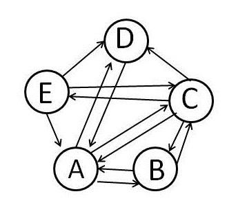
The arrow pointing from C to D means that Charlie's site links to Dana's, etc. For small collections of objects, graphs like this are an effective means of showing the links between sites.
| Exercise 2.7 | |
| (a) Create a linking matrix L which contains the information of which site links to which just as we did in the popularity example. Remember to normalize, and be sure that your input is exact (for example, make sure you enter 1/3 instead of .333 - this is important for part b, since our columns must sum to 1). Include all input and output from Matlab. | |
| (b) Use the rref command to find all solutions x to the matrix equation (L - I)x = 0. Include all input and output from Matlab (If you get something like "Empty matrix: 5-by-0", be sure to double check your answer to part a!). | |
| (c) Whose website has the highest PageRank? Explain your answer, especially in light of any negative numbers which may have arisen in part (b). List the remaining websites in order of decreasing PageRank. | |
2.5 Conclusion
Systems of linear equations, though quite uncomplicated theoretically, show up in many interesting applications. Leontief's closed exchange model and Google's Page Rank algorithm are only two of many such applications. Because systems of linear equations that arise in applications tend to be quite big and messy and not suitable to working with by hand, computer programs, such as MATLAB, turn out to be an indispensable tool for people who must work with such systems in their work.