§4.1 Introduction
Eigenvalues and determinants reveal quite a bit of information about a matrix. In this lab we will learn how to use MATLAB to compute the eigenvalues, eigenvectors, and the determinant of a matrix. We will also learn about diagonalization and how it can be applied to study certain problems in population dynamics.
§4.2 Determinants
As you should be aware by now, there is a nice formula for calculating the determinant of a 2x2 matrix. Even the 3x3 case is not that difficult. But as matrix size increases so does the complexity of calculating determinants. This is where MATLAB, or any other computer algebra program, comes in.
Example 4.1
Let's start by entering the following matrices into MATLAB. (You'll need to do this before proceeding with the rest of the example.)
To compute the determinants of these matrices we are going to use the command det(). That is, to compute the determinant of A we type the following
>> det(A)
MATLAB gives us 76 as the answer. Similarly we get>> det(B)
ans =
48
| Exercise 4.1 | |
| (a)
Use MATLAB to compute the determinants of the following matrices:
A + B, A - B, AB, A-1, BT Recall: In MATLAB the transpose of a matrix is denoted with an apostrophe; i.e. BT is given by the command >> B' |
|
| (b) Which of the above matrices are NOT invertible? Explain your reasoning. | |
| (c) Now we know the determinants of A and B, but suppose that we lost our original matrices A and B. Which of the determinants in part (a) will we still be able to recover, even without having A or B at hand? Explain your reasoning. | |
Remark 4.1 The main use of determinants in this class relates to the idea of invertibility. When you use MATLAB for that purpose, you have to understand that the program introduces rounding errors. Therefore, there is a possibility that a matrix may appear to have zero determinant and yet be invertible. This only applies to matrices with non-integer entries. The above matrices don't fall into this category as all their entries are integers.
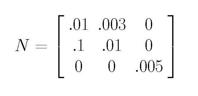
| Exercise 4.2 In
this exercise we are going to work with the following matrix:
Use det() to compute the determinant of N100. Do you think that N100 is invertible? Also use the command to compute the determinant of N. Now, using the determinant of N as a known quantity, calculate by hand the determinant of N100. Would you now reconsider your answer to the previous question? Explain. Hint: look at Remark 4.1 and consider some of the properties of determinants. |
§4.3 Eigenvalues and Eigenvectors
Given a matrix A, recall that an eigenvalue of A is a number λ such that Av = λv for some vector v. The vector v is called an eigenvector corresponding to the eigenvalue λ. Generally, it is rather unpleasant to compute eigenvalues and eigenvectors of matrices by hand. Luckily MATLAB has a function eig() that performs this task for us.
Example 4.2
Compute the eigenvalues of the matrix B from example 4.1 and assign the values to a vector b.
We do this by typing the following:
>> b = eig(B)
b =
1
8
3
2
The eigenvalues are 1, 8, 3, 2. There are four of them because our matrix is 4x4. Notice also that it is very easy to compute the determinant of B. All we have to do is multiply all the eigenvalues together. Clearly 48 = 1*8*3*2. (Further information about this can be found in your linear algebra book, Linear Algebra and Its Applications by D. Lay, in chapter 5 section 2.)
If we wanted to compute the eigenvalues of B together with the corresponding eigenvectors we would type in the following command:
>> [P,D] = eig(B)
P =
1.0000
-0.1980 0.2357 0.9074
0 0.6931
-0.2357 -0.1815
0 0.6931
0.9428 0.3630
0 0
0 0.1089
D =
1 0 0 0
0 8 0 0
0 0 3 0
0 0 0 2
MATLAB returns the matrix P consisting of the eigenvectors of B as its columns and a diagonal matrix D with the corresponding eigenvalues along the diagonal. So in the example above, the vector (-0.1980, 0.6931, 0.6931, 0)T, which is in the second column of P, is the eigenvector of B corresponding to the eigenvalue 8 which is the second entry on the diagonal of D.
Let's do a quick check of MATLAB's output and our own understanding. Enter the following command into MATLAB:
>> x = P(:,2);
This will store the second column of P, that is, the second eigenvector of P. Now enter the following in MATLAB:
>> B*x - 8*x
The output shows that Bx = 8x, which we would expect, since x is the eigenvalue of B corresponding to the eigenvalue 8.
The next exercise demonstrates a rather amazing property eigenvalues and eigenvectors to diagonalization.
| Exercise 4.3 | |
| (a) Enter
the following matrix V into
MATLAB:
>> V
= [9 -4 -2 0; Now use MATLAB to find the eigenvectors and corresponding eigenvalues of V. Assign them to matrices P and D respectively. |
|
| (b) Determine if V is invertible by looking at the eigenvalues. Explain your reasoning. | |
| (c) Use MATLAB to evaluate P-1VP. What do you notice? | |
§4.4 Diagonalization
A matrix A is called diagonalizable, if we can find an invertible matrix P such that P-1AP is diagonal. This idea may seem quite arbitrary to you; after all, why would anyone want to modify the matrix A in such a manner just to make it diagonal? To give you some idea as to why we would want to do this, consider the problem of raising some matrix A to a large power, say 100. We could, of course, multiply A by itself 100 times, but that would be rather time-consuming and ineffective. Instead, if we could express A as PDP-1, where D is a diagonal matrix and P is some invertible matrix, then, we could significantly simplify our work by noting that
A100 = (PDP-1)100 = (PDP-1)(PDP-1)(PDP-1)...(PDP-1) = PD(P-1P)D(P-1P)D(P-1P)...(P-1P)DP-1 = PD100P-1.
The upshot of this computation is that dealing with D100 is much easier than with A100 because to raise a diagonal matrix to a power, we simply raise all of its entries to that power. Thus, there is no need to perform as many matrix multiplications.
Not every matrix is diagonalizable, however. In order to diagonalize an n x n matrix A we must find a basis of Rn consisting of eigenvectors of A. Then forming a matrix P whose columns are the elements of this basis, we get P-1AP = D, where D is a diagonal matrix whose entries on the diagonal are the eigenvalues of A corresponding to the eigenvectors in the respective columns of P. If Rn does not possess such a basis of eigenvectors, then A is not diagonalizable.
In some situations, we can mak use of the following theorem:
Theorem: If an nxn matrix has n distict eigenvalues the matrix is diagonalizable.
Note, however, if the matrix does not have n distict eigenvalues this theorem does not give us any information; other means are needed to determine if is diagonalizable or not.Remark 4.2 Part (a) of the preceding exercise says that if a matrix has distinct eigenvalues, then it is diagonalizable. Note that the converse to this statement is not necessarily true; i.e., if a matrix is diagonalizable, it is not necessarily true that all its eigenvalues are distinct. A matrix can be diagonalizable even if it has repeated eigenvalues: think about the identity matrix (already diagonal) whose eigenvalues are all 1.
| Exercise 4.4 | |
| (a) Let F =
0 1 1 1 Use MATLAB to find an invertible matrix P and a diagonal matrix D such that PDP-1 = F |
|
| (b) Use MATLAB to compare F10 and PD10P-1. | |
| (c) Let f = (1,1)T. Compute Ff, F2f, F3f, F4f, F5f. Describe the pattern in your answers. | |
| (d) Given a sequence of numbers {1, 1, 2, 3, 5, 8, 13, ....} where each term is the sum of the previous two, find the 30th term of this sequence. (If you are stuck, read the remark below) | |
Remark 4.3 The sequence in the above exercise is called a Fibonacci sequence. It has many interesting properties and appears often in nature. The above problem points in the direction of how to find an explicit formula for the nth term in this sequence (it is not obvious a priori that such a formula must even exist). To obtain this formula simply note that if we let
f0 = f1 = 1 and fn+2 = fn+1 + fn
be our Fibonacci sequence and let
f = ( f0, f1)T = (1, 1)T, then
Ff = ( f1, f0 + f1)T = ( f1, f2)T,
F2f = F(Ff) = F*( f1, f2)T = (f2, f1 + f2)T = (f2, f3)T and in general,
Fnf= (fn, fn+1)T
Thus, to get the general formula we need to compute Fn, (which is done by computing PDnP-1), multiply it by the vector (1, 1)T and read off the first row of the resulting vector. If you like, you may perform these calculations by hand at your leisure and derive an interesting formula for the nth Fibonacci number involving the golden ratio.
§4.5 Returning to: Matrices and Presidential Elections
At the end of the last lab, we said that we would revisit our election example once we had a bit more mathematics under our belts. We have included the text from last time in case you want a review. If you feel confident on our work from last time, feel free to skip this review. You will need the results of the exercise from last time, so if you didn't save them, it would be helpful to rework them before moving on.
REVIEW:Certainly, the title of this section sounds a bit strange. What do matrices and presidents have in common? Let us consider a math model which is used in many subjects involving dynamics by illustrating it in a simple "sociological" situation. In California when you register to vote you declare a party affiliation. Suppose we have four political parties: Democrats, Republicans, Independents, and Libertarians, and we get the (publically available) data telling us what percentage of voters in each party switch to a different party every 4 years. So we may be told something like this... "81% of Democrats remain Democrats, 9% convert to Republicans, 6% switch to Independents and 4% become Libertarians." Suppose we have this sort of information for each party, and we organize it into a matrix, which we shall call P, as follows:
| Democrats | Republicans | Independents | Libertarians | |
| Democrats | 0.81 | 0.08 | 0.16 | 0.10 |
| Republicans | 0.09 | 0.84 | 0.05 | 0.08 |
| Independent | 0.06 | 0.04 | 0.74 | 0.04 |
| Libertarians | 0.04 | 0.04 | 0.05 | 0.78 |
(For example, the 0.05 in the second row and third column indicates that every four years, 5% of those calling themselves Independent will switch to the Republican party.) Note that we are assuming that these percentages do not change from one election to the next. This is not a very realistic assumption, but it will do for our simple model.
The question of course is to try to determine the outcome of all future elections, and if possible, the composition of the electorate in the long term. Let D0, R0, I0 and L0 denote the current percentage of Democrats, Republicans, Independents and Libertarians. In four years these numbers will change according to the matrix above, as follows:
D1 =
0.81D0 +
0.08R0 +
0.16I0 +
0.10L0
R1 =
0.09D0 +
0.84R0 +
0.05I0 +
0.08L0
I1 =
0.06D0 +
0.04R0 +
0.74I0 +
0.04L0
L1 =
0.04D0 +
0.04R0 +
0.05I0 +
0.78L0
Let xn be the vector (Dn, Rn, In, Ln)T. It represents the percentage of representatives of each party after n presidential elections and we shall call it the party distribution. From the calculation above we see that
x1 = Px0
x2 = P2x0 and in general xn = Pnx0
Assuming everyone voted along party lines, from the presidential election of 2004 we know that x0 is roughly (48.56, 51.01, 0.13, 0.30)T
| Review Exercise (you do not need to turn in, but you may need the results) | |
| (a) Enter
the matrix P and
the vector x0 into
MATLAB. To avoid mistakes, just copy and paste this:
>> P
= [0.8100 0.0800 0.1600 0.1000; >> x0 = [48.56; 51.01; 0.13; 0.30] What will the party distribution vector be 3, 7, and 10 presidential elections from now? |
|
| (b)
What will be the results 30, 60, 100 elections from now? How much different is x 30 from x 60 from x 100 ? Summarize simply what is happening with x k as k gets big. |
|
From the previous exercise you probably observed that the results seem to stabilize the further into the future we go. Let us try to explain this mathematically.
| Exercise 4.5 | |
| (a) First of all, use MATLAB to find matrices Q and D such that QDQ-1 = P | |
(b)
Now, recall that Pn = QDnQ-1.
Find  by
hand. You have probably never computed a limit of matrix
multiplication before, so just recall that our limit is simply
what the product Dn tends
to a n gets
very large. What is this limit? by
hand. You have probably never computed a limit of matrix
multiplication before, so just recall that our limit is simply
what the product Dn tends
to a n gets
very large. What is this limit? |
|
(c) Now,
using MATLAB, multiply your answer by Q and Q-1 to compute  .
Store the answer in a variable called Pinf. .
Store the answer in a variable called Pinf. |
|
| (d) Use MATLAB to compute P∞ x0 = Pinf*x0, where x0 is the same as in part (a) of the review exercise. How does your answer compare to part (b) of the review exercise from last time? | |
| (e) Now make up any vector y in R4 whose entries sum to 100. Compute P∞ y and compare it to part (d). How does the initial distribution y of the electorate seem to affect the distribution in the long term? By looking at the matrix P∞, give a mathematical explanation. | |
In Lab 2 we initially discussed Google's PageRank algorithm for ranking websites where the linking information is stored in a linking matrix L. It turns out that Google does not try to solve the problem using the methods we implemented in that lab. Here we will revisit PageRank to highlight the actual method used to solve Lr =r. If at any point you need a refresher, please reference Lab 2.
Recall after setting your problem up from the network data the equations to be solved have the form
Lr =r
where r is an k-dimensional vector and L is a k x k matrix describing the network links. Since the web is huge, an important issue is: how do we solve Lr =r when k is very large? An advantage is that most entries of L equal 0, but how do we take advantage of that? Our favorite technique so far, Gaussian elimination (or row reduction), will destroy much of this 0 structure after only a few steps, so we had better try something else. One approach goes back to
Theorem (Perron-Frobenius) If a matrix L has only non-negative entries and each of its columns sum to 1, then its largest eigenvalue is 1. Moreover, for any vector r0 with positive entries the vector rn = Ln*r0 approaches a non-negative vector r which is a solution to the eigenvalue problem Lr = r.
This is not exactly the Perron-Frobenius theorem you saw in Lab 2, but it is a variation on it. In fact, most people think of the phenomenon behind Page Rank as one of eigenvectors and eigenvalues (which we suppressed in Lab 2 because you had not yet heard of them).
This gives an alternative approach to solving Lr=r. Specifically, if we take n to be large enough, Lnr0 will approach the solution to Lr = r. As an exercise consider
The letters along the left and top are simply labels for the websites, and should not be considered part of the linking matrix. Enter this matrix into MATLAB with the command
>> L
= [0,0,0,0,1,0,0,0;
0,0,0,0,0,0,0,1;
0,1/2,0,0,0,0,1,0;
1/2,0,1/2,0,0,0,0,0;
0,0,1/2,0,0,1,0,0;
1/2,0,0,0,0,0,0,0;
0,1/2,0,0,0,0,0,0;
0,0,0,1,0,0,0,0;]
| Exercise 4.6 | |
| (a) Let e0 = [1;1;1;1;1;1;1;1], and let en+1 = L*en. (Note this is the same as saying en=Ln*e0). Compute e10. How large must n be so that enchanges by less than 1% when we increase n by 1? Don't try to get an exact value, instead just try to get a value for n that is big enough. | |
| (b) Draw by hand on your paper the graph of the network of webpages corresponding to L. (By graph here, we mean a set of vertices and edges) | |
| (bonus) This part will not be graded, but you are encouraged to do it if you find the PageRank application interesting. The question now is: what is the computational cost of solving Lr=r using iteration? More precisely, how many estimated operations are required to find rn in this method? Hint: multiplying 0 times a number and adding two numbers costs almost no time, so you just need to count how many times non-zero numbers are multiplied. | |
What usually happens in practice for very large L is that the convergence of en to e is very quick, indeed the size of n required for decent accuracy often does not go up rapidly with k. This is very important since the true linking matrix used for the internet will have k on the order of millions. The quick convergence is especially true if we have a good initial guess at the answer. Indeed the type of iteration you have just seen illustrates a basic idea behind solving many large scale problems, not just PageRank. Standard eigenvalue solvers and row reduction linear equation solvers such as Matlab are very reliable for modest size matrices, but start having trouble when there are more than a few hundred variables. "Iterative methods" work well with high probability, but there exist matrices which mess them up.
§4.7 Conclusion