Visualization of the electrostatic potentials
This section of the example illustrates the calculation of lower-resolution electrostatic potentials suitable for interactive display and manipulation. First, we need to calculate electrostatic potentials for the three molecules. This is done with the following APBS input file which can be downloaded here.
Example 1. PKA/balanol/complex visualization APBS input
read
    mol pqr bx6_7_lig_apbs.pqr  # Read balanol (mol 1)
    mol pqr bx6_7_apo_apbs.pqr  # Read PKA (mol 2)
    mol pqr bx6_7_bin_apbs.pqr  # Read complex (mol 3)
end
elec name bal
    mg-auto                          # Use the multigrid method
    dime 97 97 97                      # Grid dimensions
    fglen 70 70 70                      # Grid length
    fgcent mol 3                        # Center on complex
    cglen 80 80 80                      # Grid length
    cgcent mol 3                        # Center on complex
    mol 1
    lpbe
    bcfl sdh                           # Monopole boundary conditions
    ion 1 0.000 2.0                    # Zero ionic strength
    ion -1 0.000 2.0
    pdie 2.0                           # Solute dielectric
    sdie 78.00                         # Solvent dielectric
    chgm spl0                          # Charge disc method (linear)
    srfm smol                          # Smoothed molecular surface
    srad 0.0                           # Solvent radius
    swin 0.3                           # Surface cubic spline window
    sdens 10.0                         # Sphere density
    temp 298.15                        # Temperature
    gamma 0.105                        # Surface tension (in kJ/mol/A^2)
    calcenergy no
    calcforce no
    write pot dx ligand                # Write potential to ligand.dx
end
elec name pka
    mg-auto
    dime 97 97 97
    fglen 70 70 70
    fgcent mol 3
    cglen 80 80 80
    cgcent mol 3
    mol 2
    lpbe
    bcfl sdh
    ion 1 0.000 2.0
    ion -1 0.000 2.0
    pdie 2.0
    sdie 78.00
    chgm spl0
    srfm smol
    srad 0.0
    swin 0.3
    sdens 10.0
    temp 298.15
    gamma 0.105
    calcenergy no
    calcforce no
   write pot dx apo
end
elec name complex
    mg-auto
    dime 97 97 97
    fglen 70 70 70
    fgcent mol 3
    cglen 80 80 80
    cgcent mol 3
    mol 3
    lpbe
    bcfl sdh
    ion 1 0.000 2.0
    ion -1 0.000 2.0
    pdie 2.0
    sdie 78.00
    chgm spl0
    srfm smol
    srad 0.0
    swin 0.3
    sdens 10.0
    temp 298.15
    gamma 0.105
    calcenergy no
    calcforce no
    write pot dx complex
end

quit
|
$ apbs apbs-graphics.in
|
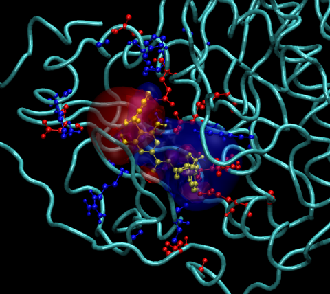
In what follows, we use the Tcl scripts my_functions and all.vmd to visualize the electrostatic potential data using VMD. The my_function Tcl script contains functions to load all 3 data sets; the user simply needs to type (at the system prompt):
$ vmd -e all.vmd
|
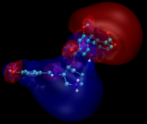
The next command loads the apo PKA electrostatic potential and is run from within VMD:
vmd > load_apo
|
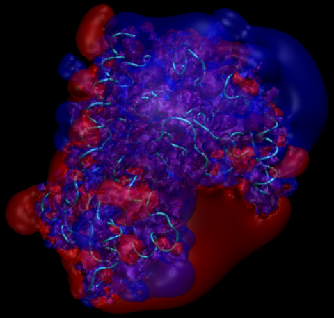
Finally, the complex can be loaded by typing, from within VMD:
vmd > load_complex
|