Statistical Models for Event-based Social Network Data
Christopher DuBois, Statistics @ UC Irvine
Carter Butts, Sociology @ UC Irvine
Daniel McFarland, Sociology @ Stanford
Padhraic Smyth, Computer Science @ UC Irvine
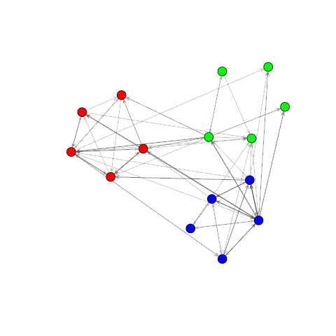
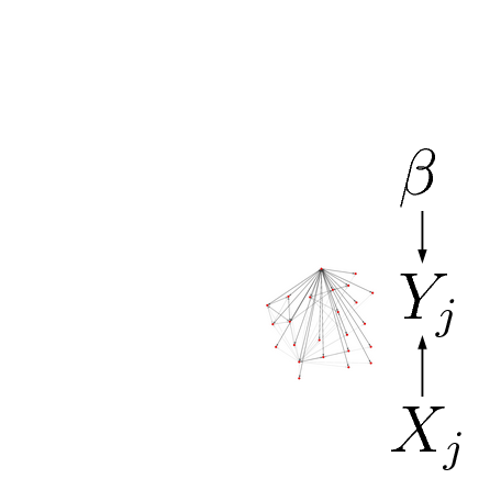
Event-based network data
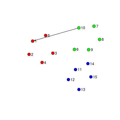
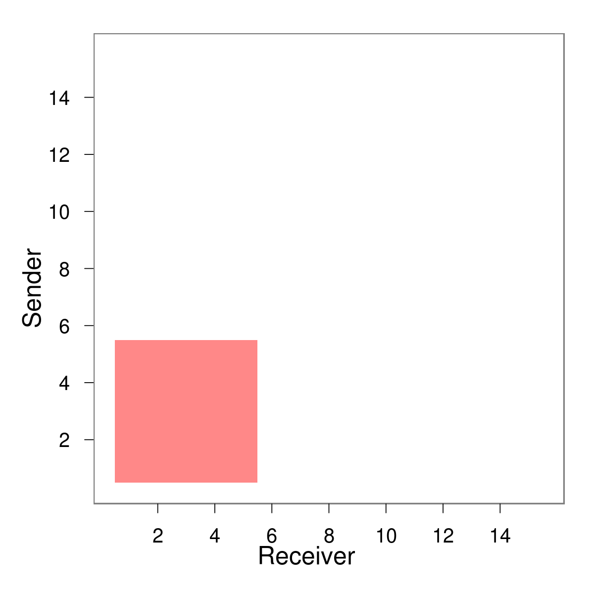
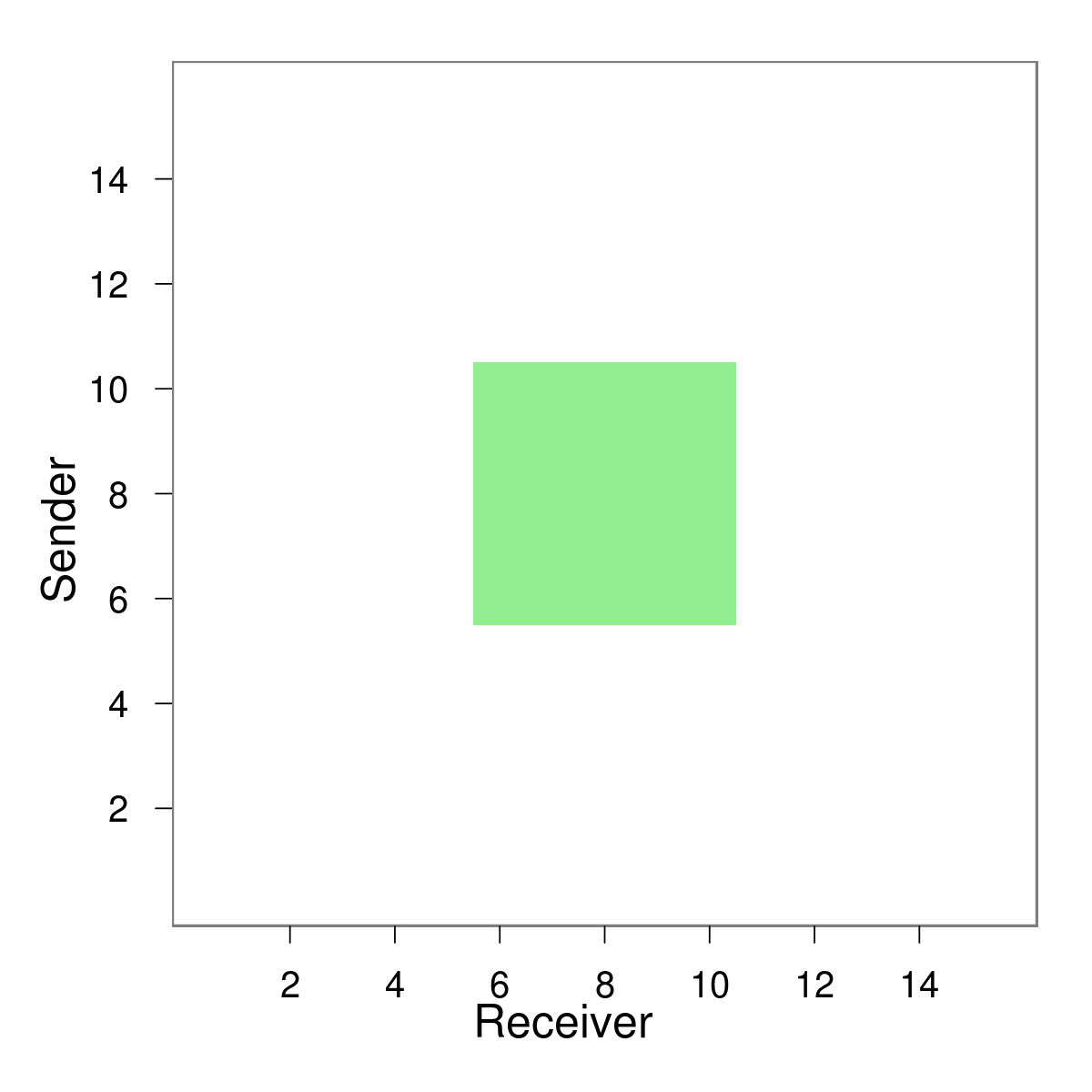
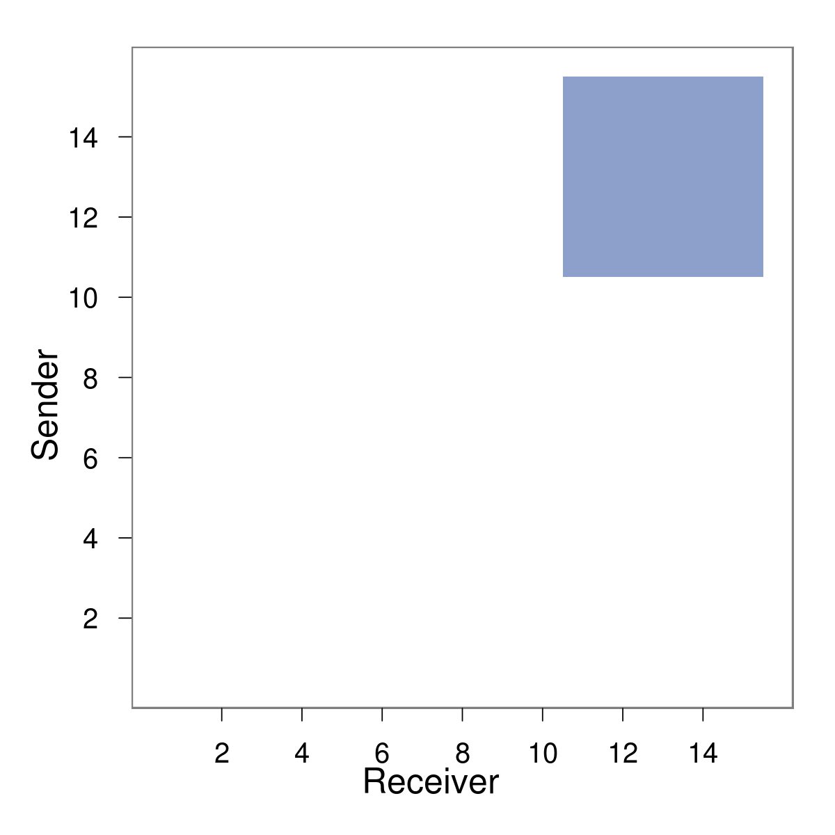
Example: Interactions among students
Communication in small groups
Modeling goals
- Dynamics of interaction in small groups
- Differential propensity to act
- Investigate association with known covariates
- regarding the individual
- previous history of events
- context
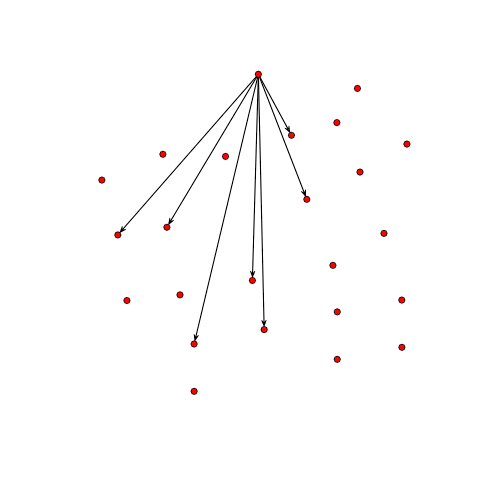
The problem of interest for today's talk involves a set of entities and events among them occurring over time. Each of these events can be called edges or relational events. One example we will return to throughout today's talk will be one where the nodes represent students in a particular classroom and the edges represent direction acts of communication. The individuals might be distinguished by some covariate, such as age, as represented by the different colors here. One of the most fundamental goals is to characterize the differential propensity to interact, and better understandhow these differences are associated with known covariates. For example, we might want to ask whether interactions between same-gender students are more likely and, furthermore, how this varies by context. To answer these types of questions, today we will discuss a statistical model for interaction in small groups of people. ----- The problem of interest for today's talk involves a set of entities and events among them occurring over time. Each event represents some interaction directed from one entity to another. I might refer to these entities as nodes, vertices, or individuals. Each of these events can be called edges or relational events. One example we will return to throughout today's talk will be one where the nodes represent students in a particular classroom and the edges represent direction acts of communication. The individuals might be distinguished by some covariate, such as age, as represented by the different colors here. This type of interaction data is of particular interest to Sociologists who study social networks and the dynamics of small groups. One of the most fundamental goals is to characterize the differential propensity to interact, and better understandhow these differences are associated with known covariates. For example, we might want to ask whether interactions between same-gender students are more likely and, furthermore, how this varies by context. To answer these types of questions, today we will discuss a statistical model for interaction in small groups of people. I will be talking about some of the challenges that arise and how we propose to solve them.
Outline
- Previous work: Models for network event data
- Background
- Relational event framework
- Simulated example
- Contribution: Hierarchical models for multiple sequences of events
- Application: High school classroom dynamics
- Future directions
Dynamic network data
"Static" analysis
Aggregate over time and analyze the weighted network
(Holland, JASA 1981) (Feinberg, JASA 1985)
Dynamic network data
"Snapshot" analysis
 Time 1 $p(Y_1 | \theta_1)$ |
 Time 2 $p(Y_2 | \theta_2)$ |
 Time t $p(Y_t | \theta_t)$ |
Dynamic network data
"Snapshot" analysis: Questions
- How do we choose the resolution for aggregating?
- A network for each day? A network for each hour?
- What happens if the behavior of interest is at a smaller time scale?
Dynamic network data
Event-level analysis
- $N$ people: $i,j \in \{1,\ldots,N\}$
- Each interaction is an edge with a timestamp: $(i,j,t)$
- Observe a sequence of edges: $\{(i_k,j_k,t_k), k\in [1,M]\}$
- Often edges can occur more than once
- Can benefit from thinking of each edge as a process with some rate
Modeling rates of events
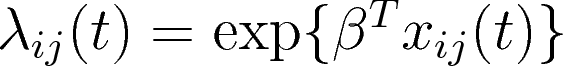
rate of interaction $(i,j)$ at time $t$
vector of covariates about $(i,j)$ at time $t$
Model rate of each edge using previous history
Modeling rates of events
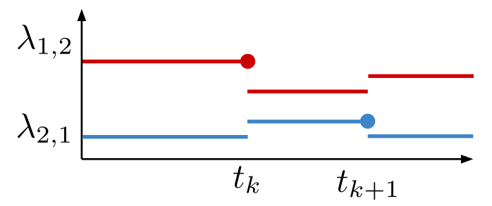
Assume event rates change only when events occur.
A relational event model

A relational event model

A relational event model
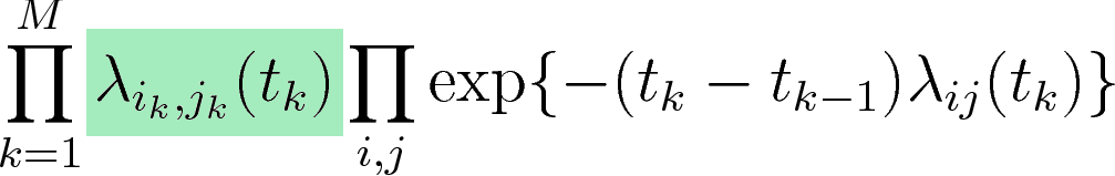
Rate of kth observed event
A relational event model
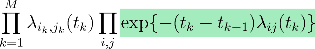
Represents the fact that no event occurred between event k-1 and event k
A relational event model
For more info see (Butts, 2008).
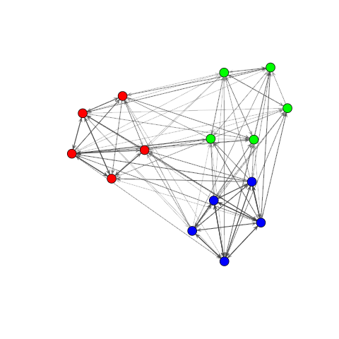
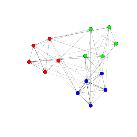
Simulation
Simulation
Model specification
$\lambda_{ij}(t) = \exp\{\beta'X_{ij}(t)\}$
Simulation
Model specification
$\log \lambda_{ij}(t) = \beta_0 + \beta_1 X_{ij1} + \beta_2 X_{ij2} + \beta_3 X_{ij3} + \beta_4 X_{ij4} + \beta_5 X_{ij5} + \beta_6 X_{ij6}$
Simulation
Model specification
$\log \lambda_{ij}(t) = \beta_0 + $ $\beta_1 X_{ij1}$$ + \beta_2 X_{ij2} + \beta_3 X_{ij3} + \beta_4 X_{ij4} + \beta_5 X_{ij5} + \beta_6 X_{ij6}$
Simulation
Model specification
$\log \lambda_{ij}(t) = \beta_0 + \beta_1 X_{ij1} + $$\ \beta_2 X_{ij2}$$ + \beta_3 X_{ij3} + \beta_4 X_{ij4} + \beta_5 X_{ij5} + \beta_6 X_{ij6}$
Simulation
Model specification
$\log \lambda_{ij}(t) = \beta_0 + \beta_1 X_{ij1} + \beta_2 X_{ij2} +$ $\ \beta_3 X_{ij3}$$ + \beta_4 X_{ij4} + \beta_5 X_{ij5} + \beta_6 X_{ij6}$
Simulation
Model specification: Participation shifts
$\log \lambda_{ij}(t) = \beta_0 + \beta_1 X_{ij1} + \beta_2 X_{ij2} + \beta_3 X_{ij3} + \beta_4 X_{ij4} + \beta_5 X_{ij5} + \beta_6 X_{ij6}$
Additive effects that model turn-taking in conversation (Gibson, 2003)
Simulation
Model specification: $(j,i)$ to $(i,j)$ effect
$\log \lambda_{ij}(t) = \beta_0 + \beta_1 X_{ij1} + \beta_2 X_{ij2} + \beta_3 X_{ij3} + $ $\ \ \beta_4 X_{ij4}$$ + \beta_5 X_{ij5} + \beta_6 X_{ij6}$
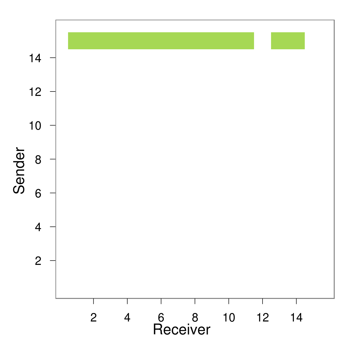
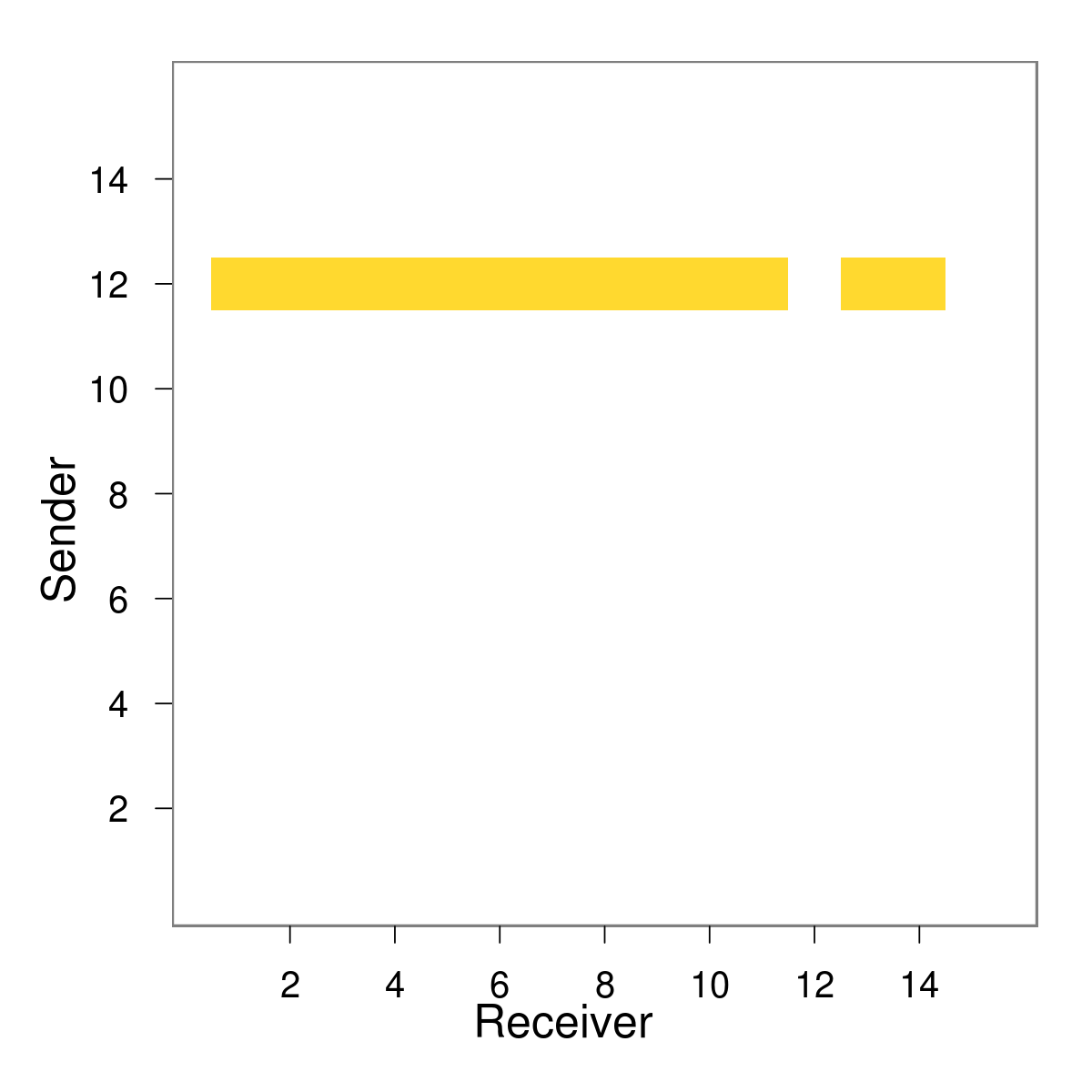
E.g. $X_{ij4}$ immediately after event (12,15)
Simulation
Model specification: $(k,i)$ to $(i,j)$ effect
$\log \lambda_{ij}(t) = \beta_0 + \beta_1 X_{ij1} + \beta_2 X_{ij2} + \beta_3 X_{ij3} + \beta_4 X_{ij4} + $ $\ \ \beta_5 X_{ij5}$$ + \beta_6 X_{ij6}$
E.g. $X_{ij5}$ immediately after event (12,15)
Simulation
Model specification: $(i,k)$ to $(i,j)$ effect
$\log \lambda_{ij}(t) = \beta_0 + \beta_1 X_{ij1} + \beta_2 X_{ij2} + \beta_3 X_{ij3} + \beta_4 X_{ij4} + \beta_5 X_{ij5} + $ $\ \ \beta_6 X_{ij6}$
E.g. $X_{ij6}$ immediately after event (12,15)
Simulation
Model specification
$\log \lambda_{ij}(t) = \beta_0 + \beta_1 X_{ij1} + \beta_2 X_{ij2} + \beta_3 X_{ij3} + \beta_4 X_{ij4} + \beta_5 X_{ij5} + \beta_6 X_{ij6}$
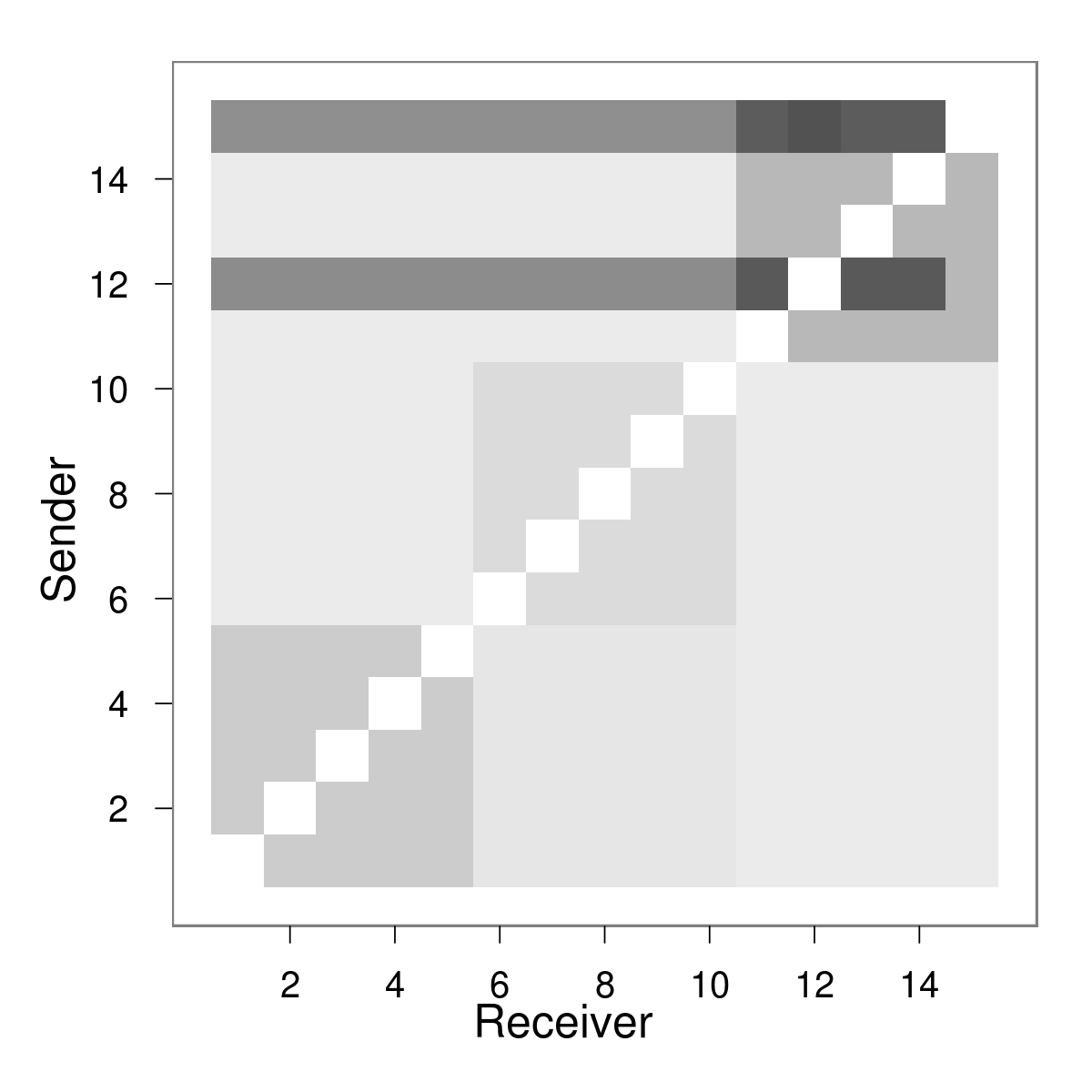
E.g. Entire matrix $\lambda$ immediately after event (12,15)
Simulation
Model specification
$\lambda_{ij}(t_k)$ |
$(i_k,j_k)$ |
Outline
- Previous work: Models for event data in networks
- Contribution: Hierarchical models for multiple sequences of events
- Motivation and specification of our hierarchical model
- Prediction experiments
- MCMC with parallel tempering
- Application: High school classroom dynamics
- Future directions
Possible issues in estimation
- Some event sequences may have few events
- Effects may have few relevant events
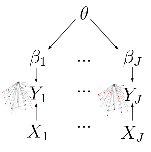
Multiple sequences
- May have a collection of event sequences
- Problem: Model applies only to a single sequence
Hierarchical event models
Proposed Contribution
- Hierarchical Bayesian model for multiple sequences
- Principled way of sharing information across sequences
- Perform population-level inferences
- Understand sequence-level variation
- Stabilize inference for poorly-constrained parameters
Hierarchical event models
Hierarchical event models
Hierarchical simulation
Parameters are Gaussians drawn from upper level
For each classroom $j$ and effect $p$:
$\begin{align}Y_j \sim& \mbox{REM}(\theta_j,\mathbf{X}_j) \\ \theta_{jp} \sim& \mbox{Normal}(\mu_p,\sigma_p^2) \\ \mu_p, \sigma_p \propto & 1/\sigma_p \end{align}$
Simulated data:
- # individuals: 15
- # sequences: 20
- $\mu_p$ as in original example
- $\sigma_p = .5$
Inference
Optimizing the posterior
$\begin{align} p(\theta,\mu,\sigma | \mathbf{Y}, \mathbf{X}) \propto & \prod_{j=1}^J \ p(Y_j|\theta_j,\mathbf{X}_j) \prod_{p=1}^P \ p(\theta_{jp}|\mu_p,\sigma_p) p(\mu_p,\sigma_p)\end{align}$
Hierarchical simulation
Learning back known parameters

Hierarchical event models
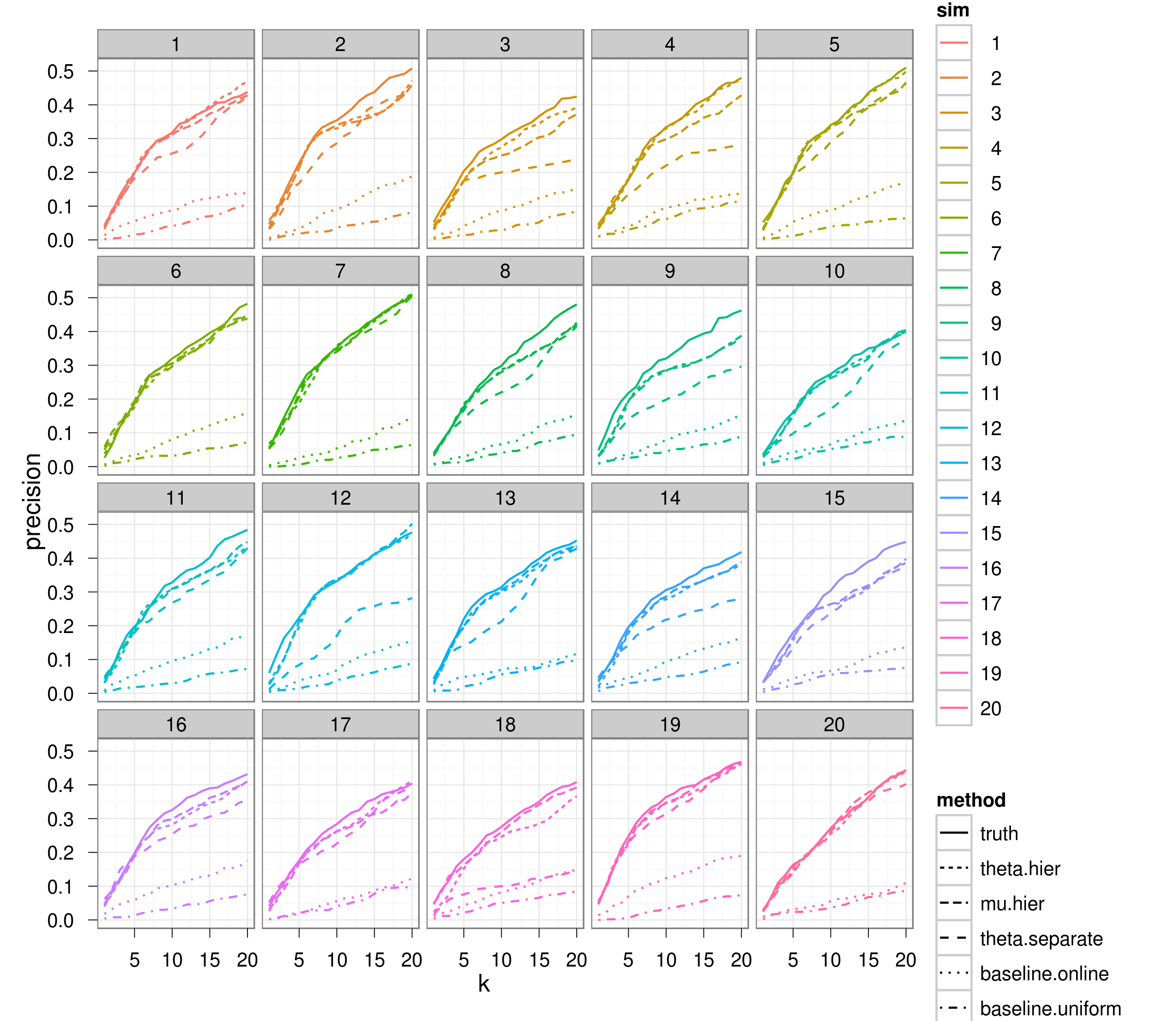
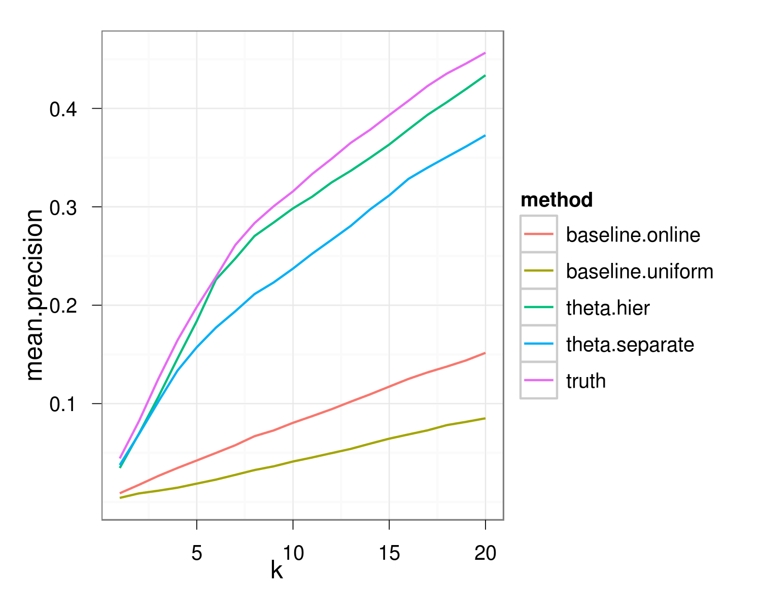
Predicting the next event
At each time $t$, rank $\lambda_{ij}(t)$
Precision @ k: Proportion of the next events that were ranked higher than k
Hierarchical event models
Predicting the next event
Inference
Markov chain Monte Carlo
- Metropolis-Hastings: construct a Markov chain whose stationary distribution is the posterior distribution of our parameters
- MH can get stuck easily: Peaked modes, some parameters might be at the boundary, and some $\theta_{jp}$ are more variable than others.
- Finding a good proposal distribution is tricky
Inference
Parallel tempering
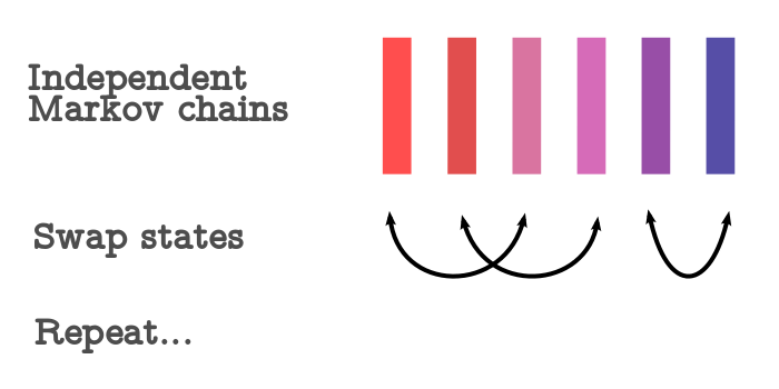
Inference
Parallel tempering
Inference
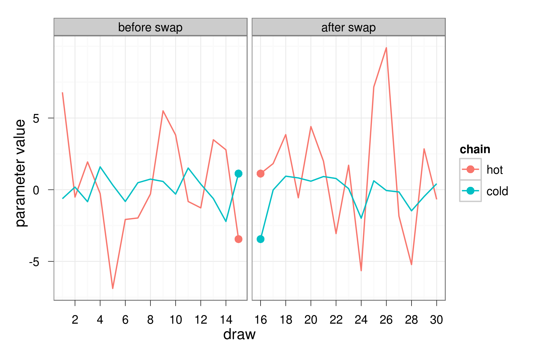
Parallel tempering: Sampling
Unnormalized distribution of interest: $g(\Theta)$
$$ \begin{align} \pi(\Theta_1,\ldots,\Theta_J) \propto& \prod_{j=1}^J h_j(\Theta_j) \\ h_j(\Theta_j) \propto & \exp \{-g(\Theta_j)/t_j \} \end{align} $$ where $t_0 < \cdots < t_J$ and $h_j(\Theta_j)$ is the target distribution for chain $j$.
Inference
Parallel tempering: Swapping
Swap between chains $j$ and $k$ at iteration $t$ with acceptance probability: $$\begin{align} \min \left\{ 1, \frac{h_j(\Theta_{k}^{(t)})h_{k}(\Theta_{j}^{(t)})}{h_j(\Theta_j^{(t)})h_{k}(\Theta_{k}^{(t)})} \right\} \end{align} $$
(Geyer 1991), (Madras 2003)
Outline
- Previous work: Models for event data in networks
- Contribution: Hierarchical models for multiple sequences of events
- Application: High school classroom dynamics
- Background
- Parameter estimates
- Model selection via DIC
- Model checking via the posterior predictive
- Future directions
Application
High school classroom data
- Collected via participant observation (McFarland, 2001)
- 650 classroom sessions
- Covariates about the class: subject, teacher, etc.
- Covariates about the individuals: race, extracurriculars, etc.
Application
High school classroom data
Model specification
Individual effects
Event effects
Participation shifts
Autocorrelation
Event context
- race
- gender
- teacher/student status
Model specification
Individual effects
Event effects
Participation shifts
Autocorrelation
Event context
- mixing terms (e.g. same sex)
- event is (teacher -> student)
- actors are friends
- number of shared activities
Model specification
Individual effects
Event effects
Participation shifts
Autocorrelation
Event context
- reciprocity (AB-BA)
- turn taking (AB-BY)
- (AB-AY), (AB-XY), (AB-BY), (AB-XA)
Model specification
Individual effects
Event effects
Participation shifts
Autocorrelation
Event context
- recency (sender/receiver)
(e.g. rank of most recent individual) - current event and previous event are both (teacher,broadcast)
Model specification
Individual effects
Event effects
Participation shifts
Autocorrelation
Event context
- Lecture
- Silent time
- Groupwork
Parameter estimation

Model selection
Deviance Information Criterion (DIC)
Deviance:
$D(y,\theta) = -2\log p(y|\theta)$
Effective # parameters:
$p_D = \frac{1}{L} \sum_{l=1}^L D(y,\theta^l) - D(y,\hat{\theta})$
Criterion:
$DIC = \frac{1}{L} \sum_{l=1}^L D(y,\theta^l) + p_D$
(Spiegelhalter,2002)
Model selection
Deviance Information Criterion (DIC)
| A | B | C | D | E | F | |
| Covs. + Recency + Pshift | 413775 | 419375 | 463227 | 484837 | 418384 | 463451 |
| Covs. + Recency | 489450 | 527203 | 546694 | 595583 | 526441 | 544513 |
| Individual mixing | X | X | X | |||
| Edgewise effects | X | X | X | |||
| Broadcast effects | X | X | X | X | ||
| Interaction w/ event context | X | X | ||||
- Participation shift effects are important
- Mixing terms important (e.g. $(i,j)$ are friends)
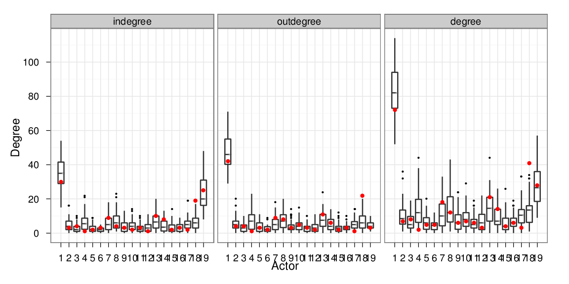
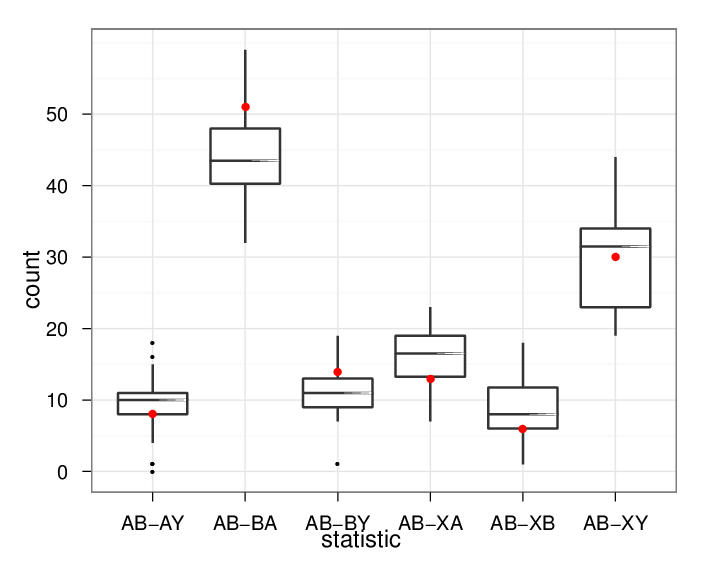
Model checking
Using the posterior predictive
- Investigate whether the observed data is reasonable under our model.
- Interested in a particular statistic of a sequence $T(Y_j)$.
- Simulate $Y_j^{(i)} \sim REM(\theta_j^{(i)},\mathbf{X}_j)$
- Compare $T(Y_j)$ to distribution of $T(Y_j^{(i)})$
Model checking
Degree distributions of a classroom session
Model checking
Participation shift statistics
Outline
- Previous work: Models for event data in networks
- Contribution: Hierarchical models for multiple sequences of events
- Application: High school classroom dynamics
- Future directions
Future work
- Model the heterogeneity among the classroom sessions
- Extend to allow for each event to include more than two individuals
Thanks
Special thanks to Carter Butts and Padhraic Smyth.
Extra slides
Alternative hierarchical structure
Using a $t$ family for $\theta$:
$\begin{align}\frac{\theta_{jp} - \mu_{p}}{\sigma_p} \sim& t_{\nu}\\ \nu \sim & \mbox{Exponential}(r)\end{align}$
Multilevel modeling
$\mu_{p} = X_j \beta_p$
Informative hyperpriors:
$\begin{align} \mu_p \sim & \mbox{Normal}(\rho,\tau)\\ \sigma_p \sim & \mbox{Gamma}(\alpha,\beta) \end{align}$
Takeaways
Parameter shrinkage
Alternative modeling choices
- Assumes exponential waiting time distribution; piecewise constant likely sufficiently flexible though. Could choose other parametric forms.
- Additive hazard model rather than multiplicative.
- Every event depends on anything in the past. Not realistic in large populations, and often not realistic for small groups.
Hierarchical normal models
Marginal posterior of tau
$\begin{align} \hat{\theta}_j =& \frac{y_{.j}/\sigma_j^2 + \mu/\tau^2}{1/(\sigma_j^2+\tau^2)} \\ \hat{v}_j =& \frac{1}{1/(\sigma_j^2+\tau^2)} \\ \hat{\mu} =& \frac{\sum_j \frac{1}{1/(\sigma_j^2+\tau^2)} y_{.j}}{\sum_j \frac{1}{1/(\sigma_j^2+\tau^2)}}\\ y_{.j} | \mu, \tau \sim & N(\mu, \sigma_j^2 + \tau^2) \\ p(\theta|\mu,\tau,y) \sim& N(\hat{\theta}_j, \hat{v}_j) \\ p(\mu,\tau|y)=&\frac{p(\mu,\tau,\theta|y)}{p(\theta|\mu,\tau,y)} \forall \theta \\ \end{align} $
Hierarchical normal models
Marginal posterior of tau
$p(\tau|y) \propto p(t) v_{\mu}^{1/2} \prod_j (\sigma_j^2 + \tau^2)^{-1/2} \exp(-(y_{.j}-\mu)^2/(2(\sigma_j^2+\tau^2)))$
Effect of hyperpriors
Only a big effect on AB-BA. Reference prior putting weight on smaller sigmas. Gamma(2,20) a strong prior, but AB-BA resisting.
Effect of hyperpriors
Under strong prior, some of the lower level effects $\theta_{jp}$ become more pronounced.
Effect of hyperpriors
Hierarchical event models
Predicting the next event