CS295 Realistic Image Synthesis
Programming Assignment 1: Monte Carlo Sampling and Direct Illumination
Instructor: Shuang Zhao
Due: Tuesday May 21, 2019 (23:59 pm Pacific Time)
Credit: The programming assignments of this course is based on Nori, an educational renderer created by Wenzel Jakob.
What to submit
- A report including results and discussions required by Part 1, 2, and 3.
- A zip package containing your nori/CMakeLists.txt file as well as full nori/include/ and nori/src/ directories.
This part of the assignment is for you to properly setup Nori and get familiar with its key components. You do NOT have to submit anything.
Part 0.1. Setting Up a C++ Compiler and Building the Base Code
Click here to download Nori's base code as well as all scene files needed for this assignment.
Linux / Mac OS X
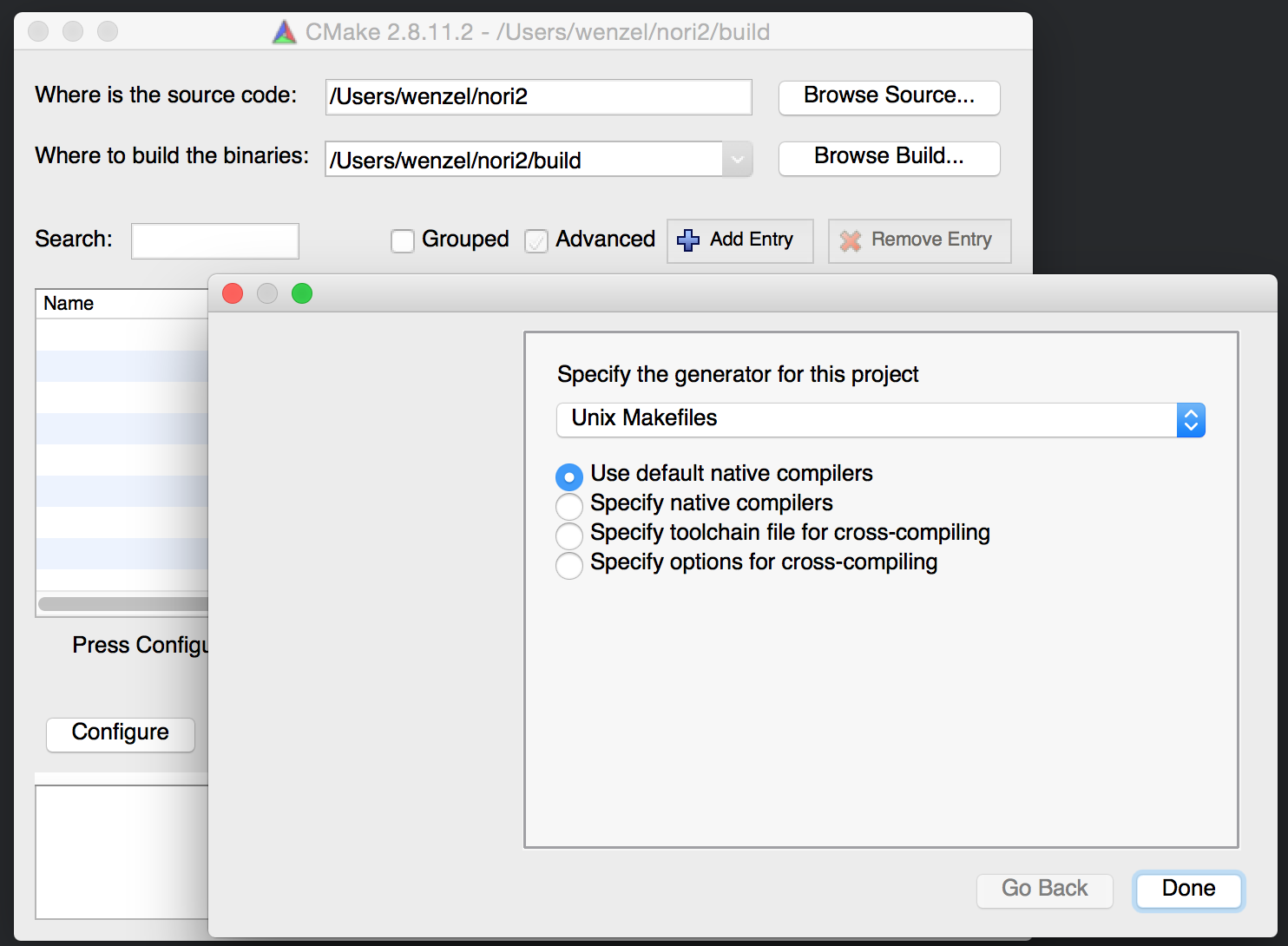
Begin by installing the CMake build system on your system. On Mac OS X, you will also need to install a reasonably up-to-date version of XCode along with the command line tools. On Linux, any reasonably recent version of GCC or Clang will work. Navigate to the Nori folder, create a build directory and start cmake-gui, like so:
$ cd path-to-nori
$ mkdir build
$ cd build
$ cmake-gui ..
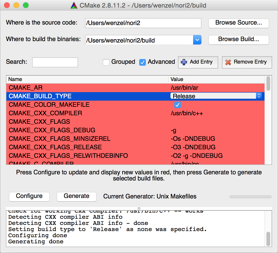
After the Makefiles are generated, simply run make to compile all dependencies and Nori itself.
$ make -j 4This can take quite a while; the above command compiles with four processors at the same time. Note that you will probably see many warning messages while the dependencies are compiled—you can ignore them.
Windows / Visual Studio 2013
Begin by installing Visual Studio 2013 (older versions won't do) and a reasonably recent version (3.x or later) of CMake. Start CMake and navigate to the Nori directory.
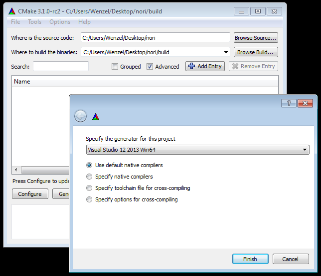
After setting up the project, click the Configure and Generate button. This will create a file called nori.sln—double-click it to open Visual Studio.
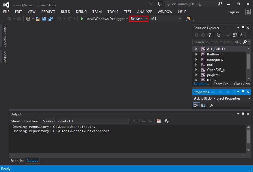
The Build->Build Solution menu item will automatically compile all dependency libraries and Nori itself; the resulting executable is written to the Release or Debug subfolder of your chosen build directory. Note that you will probably see many warning messages while the dependencies are compiled—you can ignore them.
Part 0.2. A High-Level Overview
The Nori base code consists of the base code files (left table) and several dependency libraries (right table) that are briefly explained below.| Directory | Description |
|---|---|
| src | A directory containing the main C++ source code |
| include/nori | A directory containing header files with declarations |
| ext | External dependency libraries (see the table right) |
| scenes | Example scenes and test datasets to validate your implementation |
| CMakeLists.txt | A CMake build file which specifies how to compile and link Nori |
| CMakeConfig.txt | A low-level CMake build file which specifies how to compile and link several dependency libraries upon which Nori depends. You probably won't have to change anything here. |
| Directory | Description |
|---|---|
| ext/openexr | A high dynamic range image format library |
| ext/pcg32 | A tiny self-contained pseudorandom number generator |
| ext/filesystem | A tiny self-contained library for manipulating paths on various platforms |
| ext/pugixml | A light-weight XML parsing library |
| ext/tbb | Intel's Boost Thread Building Blocks for multi-threading |
| ext/tinyformat | Type-safe C++11 version of printf and sprintf |
| ext/hypothesis | Functions for statistical hypothesis tests |
| ext/nanogui | A minimalistic GUI library for OpenGL |
| ext/nanogui/ext/eigen | A linear algebra library used by nanogui and Nori. |
| ext/zlib | A compression library used by OpenEXR |
Eigen
When developing any kind of graphics-related software, it's important to be familiar with the core mathematics support library that is responsible for basic linear algebra types, such as vectors, points, normals, and linear transformations. Nori uses Eigen 3 for this purpose. We don't expect you to understand the inner workings of this library but recommend that you at least take a look at the helpful tutorial provided on the Eigen web page.
Nori provides a set of linear algebra types that are derived from Eigen's matrix/vector class (see e.g. the header file include/nori/vector.h). This is necessary because we will be handling various quantities that require different treatment when undergoing homogeneous coordinate transformations, and in particular we must distinguish between positions, vectors, and normals. The main subset of types that you will most likely use are:
- Point2i,
- Point2f,
- Point3f,
- Vector2i,
- Vector2f,
- Vector3f, and
- Normal3f.
pugixml
The pugixml library implements a tiny XML parser that we use to load Nori scenes. The format of these scenes is described below. The XML parser is fully implemented for your convenience, but you may have to change it if you wish to extend the file format for your final project.
pcg32
PCG is a family of tiny pseudo-random number generators with good performance that was recently proposed by Melissa O'Neill. The full implementation of pcg32 (one member of this family) is provided in a single header file in ext/pcg32/pcg32.h. You will be using this class as a source of pseudo-randomness.
Hypothesis test support library
With each programming assignment, we will provide statistical hypothesis tests that you can use to verify that your algorithms are implemented correctly. You can think of them as unit tests with a little extra twist: suppose that the correct result of a certain computation in a is given by a constant \(c\). A normal unit test would check that the actual computed \(c'\) satisfies \(|c-c'|<\varepsilon\) for some small constant \(\varepsilon\) to allow for rounding errors etc. However, rendering algorithms usually employ randomness (they are Monte Carlo algorithms), and in practice the computed answer \(c'\) can be quite different from \(c\), which makes it tricky to choose a suitable constant \(\varepsilon\).
A statistical hypothesis test, on the other hand, analyzes the computed value and an estimate of its variance and tries to assess how likely it is that the difference \(|c-c'|\) is due to random noise or an actual implementation bug. When it is extremely unlikely (usually \(p<0.001\)) that the error could be attributed to noise, the test reports a failure.
OpenEXR
OpenEXR is a standardized file format for storing high dynamic range images. It was originally developed by Industrial Light and Magic and is now widely used in the movie industry and for rendering in general. The directory ext/openexr contains the open source reference implementation of this standard. You will probably not be using this library directly but through Nori's Bitmap class implemented in src/bitmap.cpp and include/nori/bitmap.h to load and write OpenEXR files.
NanoGUI
The NanoGUI library creates an OpenGL window and provides a small set of user interface elements (buttons, sliders, etc.). We use it to show the preview of the image being rendered. This library could be useful if your final project involves some kind of user interaction.
Intel Thread Building Blocks
The tbb directory contains Intel's Thread Building Blocks (TBB). This is a library for parallelizing various kinds of programs similar in spirit to OpenMP and Grand Central Dispatch on Mac OS. You will see in the course that renderings often require significant amounts of computation, but this computation is easy to parallelize. We use TBB because it is more portable and flexible than the aforementioned platform-specific solutions. The basic rendering loop in Nori (in src/main.cpp) is already parallelized, so you will probably not have to read up on this library unless you plan to parallelize a custom algorithm for your final project.
Part 0.3. Scene File Format and Parsing
Take a moment to browse through the header files in include/nori. You will generally find all important interfaces and their documentation in this place. Most headers files also have a corresponding .cpp implementation file in the src directory. The most important class is called NoriObject—it is the base class of everything that can be constructed using the XML scene description language. Other interfaces (e.g. Camera) derive from this class and expose additional more specific functionality (e.g. to generate an outgoing ray from a camera).
Nori uses a very simple XML-based scene description language, which can be interpreted as a kind of building plan: the parser creates the scene step by step as it reads the scene file from top to bottom. The XML tags in this document are interpreted as requests to construct certain C++ objects including information on how to put them together.
Each XML tag is either an object or a property. Objects correspond to C++ instances that will be allocated on the heap. Properties are small bits of information that are passed to an object at the time of its instantiation. For instance, the following snippet creates red diffuse BSDF:
<bsdf type="diffuse">
    <color name="albedo" value="0.5, 0, 0"/>
</bsdf>
Here, the <bsdf> tag will cause the creation of an object of type BSDF, and the type attribute specifies what specific subclass of BSDF should be used. The <color> tag creates a property of name albedo that will be passed to its constructor. If you open up the C++ source file src/diffuse.cpp, you will see that there is a constructor, which looks for this specific property:
Diffuse(const PropertyList &propList) {
    m_albedo = propList.getColor("albedo", Color3f(0.5f));
}
The piece of code that associates the "diffuse" XML identifier with the Diffuse class in the C++ code is a macro found at the bottom of the file:
NORI_REGISTER_CLASS(Diffuse, "diffuse");
Certain objects can be nested hierarchically. For example, the following XML snippet creates a mesh that loads its contents from an external OBJ file and assigns a red diffuse BRDF to it.
<mesh type="obj">
    <string type="filename" value="bunny.obj"/>

    <bsdf type="diffuse">
        <color name="albedo" value="0.5, 0, 0"/>
    </bsdf>
</mesh>
Implementation-wise, this kind of nesting will cause a method named addChild() to be invoked within the parent object. In this specific example, this means that Mesh::addChild() is called, which roughly looks as follows:
void Mesh::addChild(NoriObject *obj) {
    switch (obj->getClassType()) {
        case EBSDF:
            if (m_bsdf)
                throw NoriException(
                    "Mesh: multiple BSDFs are not allowed!");
            /// Store pointer to BSDF in local instance
            m_bsdf = static_cast<BSDF *>(obj);
            break;
    // ..(omitted)..
}
This function verifies that the nested object is a BSDF, and that no BSDF was specified before; otherwise, it throws an exception of type NoriException.
The following different types of properties can currently be passed to objects within the XML description language:
<!-- Basic parameter types -->
<string name="property name" value="arbitrary string"/>
<boolean name="property name" value="true/false"/>
<float name="property name" value="float value"/>
<integer name="property name" value="integer value"/>
<vector name="property name" value="x, y, z"/>
<point name="property name" value="x, y, z"/>
<color name="property name" value="r, g, b"/>
<!-- Linear transformations use a different syntax -->
<transform name="property name">
    <!-- Any sequence of the following operations: -->
    <translate value="x, y, z"/>
    <scale value="x, y, z"/>
    <rotate axis="x, y, z" angle="deg."/>
    <!-- Useful for cameras and spot lights: -->
    <lookat origin="x,y,z" target="x,y,z" up="x,y,z"/>
</transform>
The top-level element of any scene file is usually a <scene> tag, but this is not always the case. For instance, some of the programming assignments will ask you to run statistical tests on BRDF models or rendering algorithms, and these tests are also specified using the XML scene description language, like so:
<?xml version="1.0"?>

<test type="chi2test">
    <!-- Run a χ2 test on the microfacet BRDF model (@ 0.01 significance level) -->
    <float name="significanceLevel" value="0.01"/>

    <bsdf type="microfacet">
        <float name="alpha" value="0.1"/>
    </bsdf>
</test>
Part 0.4. Creating Your First Nori Class
In Nori, rendering algorithms are referred to as integrators because they generally solve a numerical integration problem. The remainder of this section explains how to create your first (dummy) integrator which visualizes the surface normals of objects.
We begin by creating a new Nori object subclass in src/normals.cpp with the following content:
#include <nori/integrator.h>
NORI_NAMESPACE_BEGIN
class NormalIntegrator : public Integrator {
public:
NormalIntegrator(const PropertyList &props) {
m_myProperty = props.getString("myProperty");
std::cout << "Parameter value was : " << m_myProperty << std::endl;
}
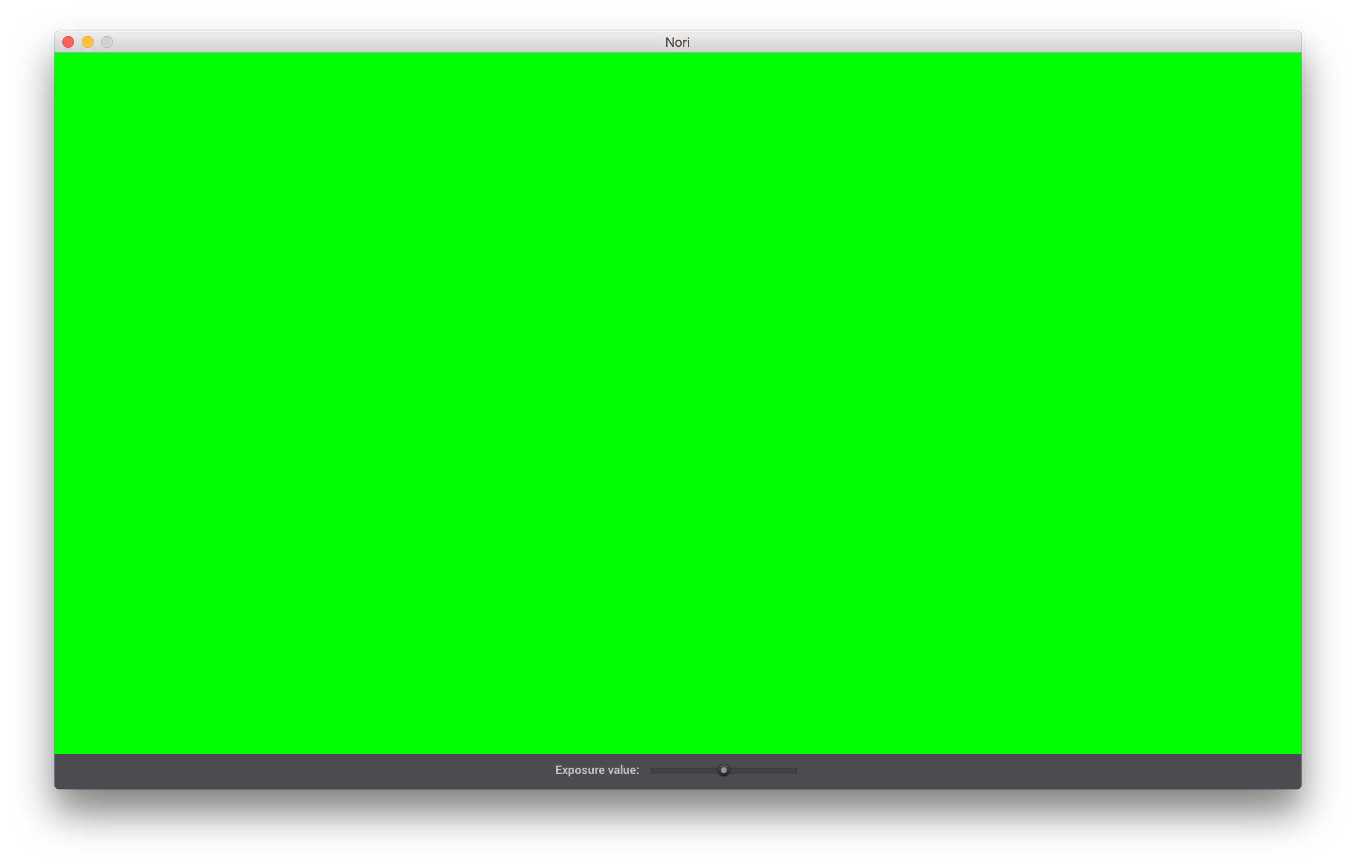
/// Compute the radiance value for a given ray. Just return green here
Color3f Li(const Scene *scene, Sampler *sampler, const Ray3f &ray) const {
return Color3f(0, 1, 0);
}
/// Return a human-readable description for debugging purposes
std::string toString() const {
return tfm::format(
"NormalIntegrator[\n"
" myProperty = \"%s\"\n"
"]",
m_myProperty
);
}
protected:
std::string m_myProperty;
};
NORI_REGISTER_CLASS(NormalIntegrator, "normals");
NORI_NAMESPACE_END
To try out this integrator, we first need to add it to the CMake build system: for this, open CMakeLists.txt and look for the command
add_executable(nori,
  # Header files
  include/nori/bbox.h
  ...

  # Source code files
  src/bitmap.cpp
  ...
)
Add the line src/normals.cpp at the end of the source file list and recompile. If everything goes well, CMake will create an executable named nori (or nori.exe on Windows) which you can call on the command line.
Finally, create a small test scene with the following content and save it as test.xml:
<?xml version="1.0"?>

<scene>
    <integrator type="normals">
        <string name="myProperty" value="Hello!"/>
    </integrator>

    <camera type="perspective"/>
</scene>
This file instantiates our integrator and creates the default camera setup. Running nori with this scene causes two things to happen:
$ ./nori test.xml

Property value was : Hello!

Configuration: Scene[
  integrator = NormalIntegrator[
    myProperty = "Hello!"
  ],
  sampler = Independent[sampleCount=1]
  camera = PerspectiveCamera[
    cameraToWorld = [1, 0, 0, 0;
                     0, 1, 0, 0;
                     0, 0, 1, 0;
                     0, 0, 0, 1],
    outputSize = [1280, 720],
    fov = 30.000000,
    clip = [0.000100, 10000.000000],
    rfilter = GaussianFilter[radius=2.000000, stddev=0.500000]

  ],
  medium = null,
  envEmitter = null,
  meshes = {
  }
]

Rendering .. done. (took 93.0ms)
Writing a 1280x720 OpenEXR file to "test.exr"
The Nori executable echoed the property value we provided, and
it printed a brief human-readable summary of the scene.
The rendered scene is saved as an OpenEXR file named test.exr.
Visualizing OpenEXR files
A word of caution: various tools for visualizing OpenEXR images exist, but not all really do what one would expect. Adobe Photoshop and the HDRITools by Edgar Velázquez-Armendáriz work correctly, but Preview.app on Mac OS for instance tonemaps these files in an awkward and unclear way.
If in doubt, you can also use Nori as an OpenEXR viewer: simply run it with an EXR file as parameter, like so:
$ ./nori test.exr
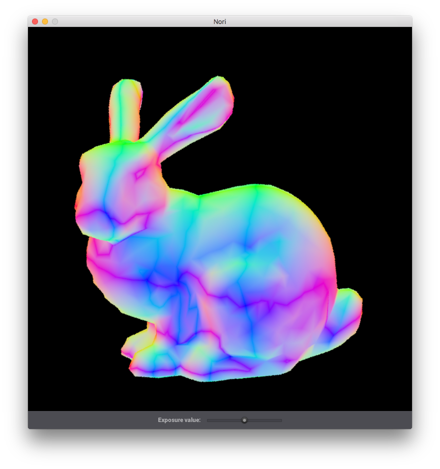
Tracing rays
Let's now build a more interesting integrator which traces some rays against the scene geometry. Change the file normals.cpp as shown on the left side. Invoke nori on the file scenes/pa1/bunny.xml, and you should get the image on the right.
#include <nori/integrator.h>
#include <nori/scene.h>

NORI_NAMESPACE_BEGIN

class NormalIntegrator : public Integrator {
public:
    NormalIntegrator(const PropertyList &props) {
        /* No parameters this time */
    }

    Color3f Li(const Scene *scene, Sampler *sampler, const Ray3f &ray) const {
        /* Find the surface that is visible in the requested direction */
        Intersection its;
        if (!scene->rayIntersect(ray, its))
            return Color3f(0.0f);

        /* Return the component-wise absolute
           value of the shading normal as a color */
        Normal3f n = its.shFrame.n.cwiseAbs();
        return Color3f(n.x(), n.y(), n.z());
    }

    std::string toString() const {
        return "NormalIntegrator[]";
    }
};

NORI_REGISTER_CLASS(NormalIntegrator, "normals");
NORI_NAMESPACE_END
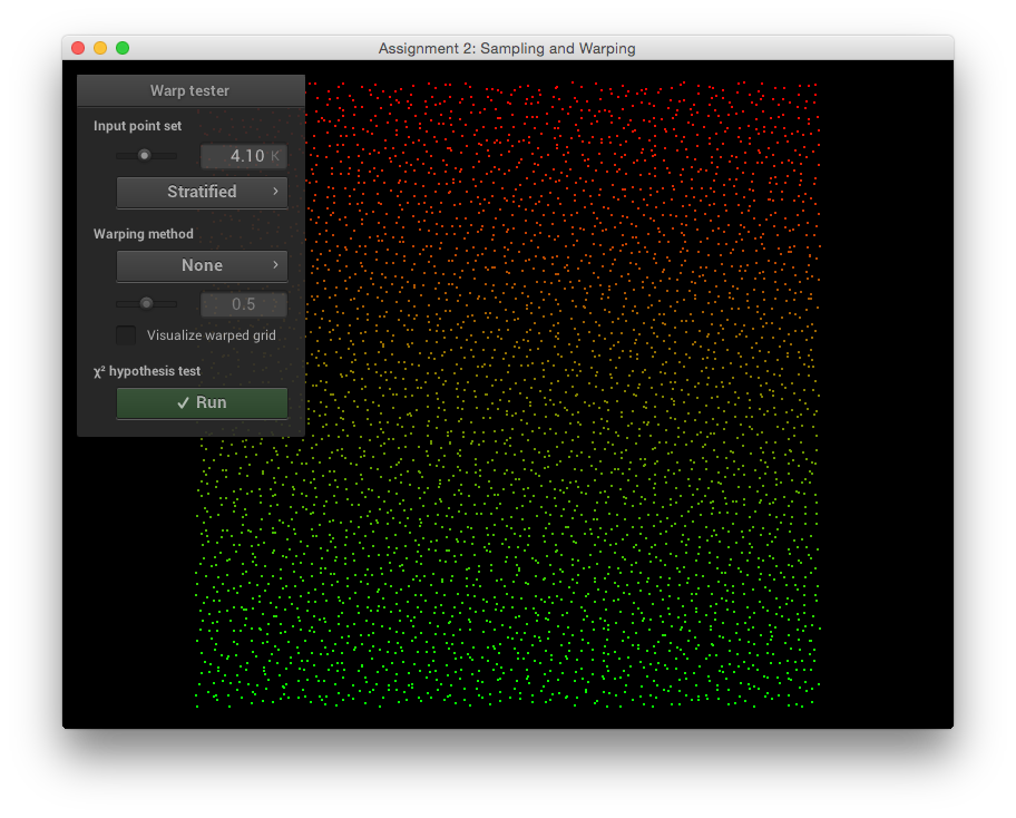
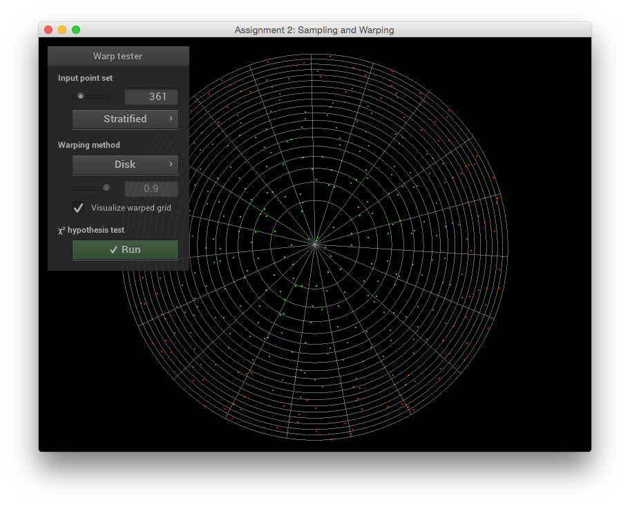
In this exercise you will generate sample points on various domains: the plane, disks, spheres, and hemispheres. The base code has been extended with an interactive visualization and testing tool to make working with point sets as intuitive as possible.
After compiling the provided base code, you should see an executable named warptest. Run this executable to launch the interactive warping tool, which allows you to visualize the behavior of different warping functions given a range of input point sets (independent, grid, and stratified). Up to now, we only discussed uniform random variables which correspond to the "independent" type, and you need not concern yourself with the others for now.
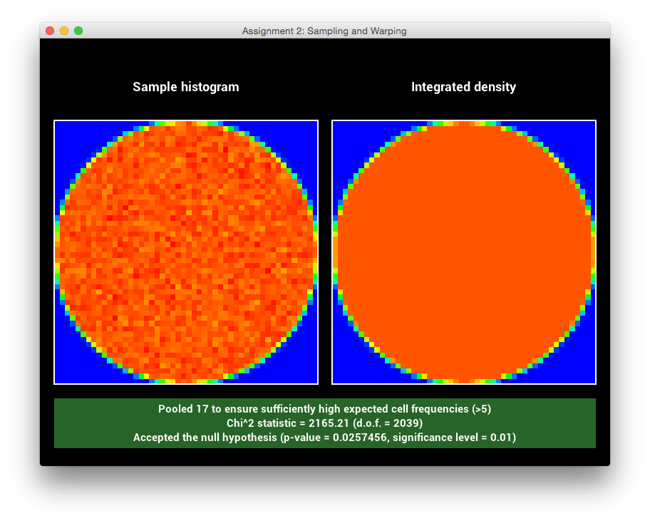
Part 1 is split into several subsections; in each case, you are asked to implement a distribution function and a matching sample warping scheme It is crucial that both are consistent with respect to each other (i.e. that warped samples have exactly the distribution described by the density function). Significant errors can arise if inconsistent warpings are used for Monte Carlo integration. The warptest tool provided by us implements a \(\chi^2\) test to ensure that this consistency requirement is indeed satisfied.
Part 1.1. Sample Warping
Implement the missing functions in class Warp found in
src/warp.cpp. This class consists of various warp methods that
take as input a 2D point \((s, t) \in [0, 1) \times [0, 1) \) and
return the warped 2D (or 3D) point in the new domain. Each method is
accompanied by another method that returns the probability density with
which a sample was picked. Our default implementations all throw an
exception, which produces an error message in the graphical user
interface of warptest. The slides on the course website
provide a number of useful recipes for warping samples and computing
the densities, and the PBRT textbook also contains considerable
information on this topic that you should feel free to use.
-
Warp::squareToTentandWarp::squareToTentPdfImplement a method that transforms uniformly distributed 2D points on the unit square into the 2D "tent" distribution, which has the following form: \[ p(x, y)=p_1(x)\,p_1(y)\quad\text{and}\quad p_1(t) = \begin{cases} 1-|x|, & -1\le x\le 1\\ 0,&\text{otherwise}\\ \end{cases} \]
Note that this distribution is composed of two independent 1D distributions, which makes this task considerably easier. Follow the "recipe" discussed in class:- Compute the CDF \(P_1(t)\) of the 1D distribution \(p_1(t)\)
- Derive the inverse \(P_1^{-1}(t)\)
- Map a random variable \(\xi\) through the inverse \(P_1^{-1}(t)\) from the previous step
-
Warp::squareToUniformDiskandWarp::squareToUniformDiskPdfImplement a method that transforms uniformly distributed 2D points on the unit square into uniformly distributed points on a planar disk with radius 1 centered at the origin. Next, implement a probability density function that matches your warping scheme.
-
Warp::squareToUniformSphereandWarp::squareToUniformSpherePdfImplement a method that transforms uniformly distributed 2D points on the unit square into uniformly distributed points on the unit sphere centered at the origin. Implement a matching probability density function.
-
Warp::squareToUniformHemisphereandWarp::squareToUniformHemispherePdfImplement a method that transforms uniformly distributed 2D points on the unit square into uniformly distributed points on the unit hemisphere centered at the origin and oriented in direction \((0, 0, 1)\). Add a matching probability density function.
-
Warp::squareToCosineHemisphereandWarp::squareToCosineHemispherePdfTransform your 2D point to a point distributed on the unit hemisphere with a cosine density function \[ p(\theta)=\frac{\cos\theta}{\pi}, \] where \(\theta\) is the angle between a point on the hemisphere and the north pole.
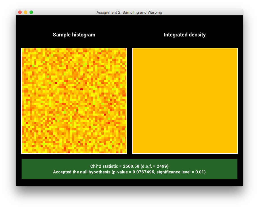
Part 1.2. Validation
Pass the \(\chi^2\) test for each one of the above sampling techniques and include screen shots in your report.
In this part of the homework, you'll implement two basic rendering algorithms that set the stage for fancier methods investigated later in the course. For now, both of the methods assume that the object is composed of a simple white diffuse material that reflects light uniformly into all directions.

Part 2.1. Point lights
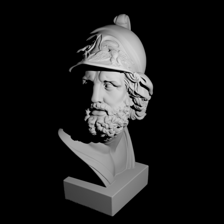
The provided base code includes a scene scenes/pa1/ajax-simple.xml that instantiates a (currently nonexistent) integrator/rendering algorithm named simple, which simulates a single point light source located at a 3D position position, and which emits an amount of energy given by the parameter energy.
<!-- An excerpt from scenes/pa1/ajax-simple.xml: -->
<integrator type="simple">
    <point name="position" value="-20, 40, 20"/>
    <color name="energy" value="3000, 3000, 3000"/>
</integrator>
Your first task will be to create a new Integrator that accepts these parameters (in a similar way as the dummy normals integrator shown at the beginning of Part 0.4).
Take a look at the PropertyList class, which should be used to extract the two parameters.
Let \(\mathbf{p}\) and \(\mathbf{\Phi}\) denote the position and energy of the light source, and suppose that \(\mathbf{x}\) is the point being rendered. Then this integrator should compute the quantity
\[ L(\mathbf{x})=\frac{\Phi}{4\pi^2} \frac{\mathrm{max}(0, \cos\theta)}{\|\mathbf{x}-\mathbf{p}\|^2} V(\mathbf{x}\leftrightarrow\mathbf{p}) \]
where \(\theta\) is the angle between the direction from \(\mathbf{x}\) to \(\mathbf{p}\) and the shading surface normal (available in Intersection::shFrame::n) at \(\mathbf{x}\) and
is the visibility function, which can be implemented using a shadow ray query. Intersecting a shadow ray against the scene is generally cheaper since it suffices to check whether an intersection exists rather than having to find the closest one.
Implement the simple integrator according to this specification and
render the scene scenes/pa1/ajax-simple.xml.
Include a comparison against the reference image in your report.
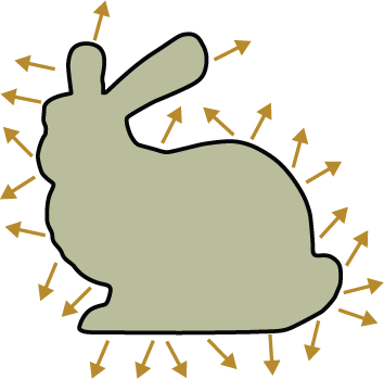
Part 2.2. Ambient occlusion
Ambient occlusion is rendering technique which assumes that a (diffuse) surface receives uniform illumination from all directions (similar to the conditions inside a light box), and that visibility is the only effect that matters. Some surface positions will receive less light than others since they are occluded, hence they will look darker. Formally, the quantity computed by ambient occlusion is defined as
\[ L(\mathbf{x})=\int_{\Omega_\mathbf{x}}V(\mathbf{x}, \mathbf{x}+\alpha\omega)\,\frac{\cos\theta}{\pi}\,\mathrm{d}\omega \]
which is an integral over the upper hemisphere \(\Omega_{\mathbf{x}}\) centered at the point \(\mathbf{x}\). The variable \(\theta\) refers to the angle between the direction \(\omega\) and the shading normal at \(\mathbf{x}\). The ad-hoc variable \(\alpha\) adjusts how far-reaching the effects of occlusion are.
Note that this situation—sampling points on the hemisphere with a cosine weight—exactly corresponds
to one of the warping functions you implemented in Part 2.1, specifically squareToCosineHemisphere. Use this function to sample a point on the hemisphere and then check for visibility
using a shadow ray query. You can assume that occlusion is a global effect (i.e. \(\alpha=\infty\)).
One potential gotcha is that the samples produced by squareToCosineHemisphere lie in the reference hemisphere and need to be oriented according to the surface at \(\mathbf{x}\). Take a look at the Frame class, which is intended to facilitate this.
Implement the ambient occlusion (ao) integrator and render the scene scenes/pa1/ajax-ao.xml.
Include a comparison against the reference image in your report.
Part 3.1. Area lights
Our first goal will be to extend Nori so that any geometric object can be turned into a light source known as an area light.
Each triangle of a mesh that is marked as an area light uniformly emits radiance towards all directions above its surface. In Nori's XML description language, area lights are specified using a nested emitter tag of type area. Here is an example:
<scene>
    <!-- Load a OBJ file named "bunny.obj" -->
    <mesh type="obj">
        <string name="filename" value="bunny.obj"/>

        <!-- Turn the mesh into an area light source -->
        <emitter type="area">
            <!-- Assign a uniform radiance of 1 W/m2sr -->
            <color name="radiance" value="1, 1, 1"/>
        </emitter>
    </mesh>

    <!-- ..... -->
</scene>
Currently, Nori won't be able to understand the above snippet since area lights are not yet implemented. To add area lights to Nori, follow these steps:
-
Create a new class
AreaLightin a file namedsrc/area.cppthat derives from theEmitterclass. Connect it to the scene parser using theNORI_*macros similar to theIntegrators you have previously created. Use the constructor'sconst PropertyList &argument to extract theradianceparameter in the constructor.
-
The Monte Carlo rendering technique in Part 3.2 requires the ability to sample points that are uniformly distributed on area lights. Currently, none of this functionality exists.
Begin by familiarizing yourself with the
Meshclass to see how vertices, faces and normals are stored. Next, add a method that uniformly samples positions on the surface associated with a specificMeshinstance. The name and precise interface of this method are completely up to you. However, we suggest that it should take a uniformly 2D sample and return:- The sampled position \(\mathbb{p}\) on the surface of the mesh.
- The interpolated surface normal \(\mathbb{n}\) at \(\mathbb{p}\) computed from the per-vertex normals. When the mesh does not provide per-vertex normals, compute and return the face normal instead.
-
The probability density of the sample. This should be the reciprocal of the surface area of the entire mesh.
You may find the
DiscretePDFclass (declared in include/nori/dpdf.h) useful to implement the sampling step. We suggest that you use this class to build a discrete probability distribution that will allow you to pick a triangle proportional to its surface area. Once a triangle is chosen, you can (uniformly) sample a barycentric coordinate \((\alpha, \beta, 1-\alpha-\beta)\) using the mapping \[ \begin{pmatrix} \alpha\\ \beta \end{pmatrix} \mapsto \begin{pmatrix} 1 - \sqrt{1 - \xi_1}\\ \xi_2\, \sqrt{1 - \xi_1} \end{pmatrix} \] where \(\xi_1\) and \(\xi_2\) are uniform variates.The precomputation to build the discrete probability distribution can be performed in the
activate()method of theMeshclass, which is automatically invoked by the XML parser.
Part 3.2. Distribution Ray Tracing
In this part you will implement a new direct illumination integrator, which integrates the incident radiance by sampling points on a set of emitters (a.k.a. light sources). Emitters can be fully, partially or not at all visible from a point in your scene, hence you will need to perform Monte Carlo integration to compute the reflected radiance while accounting for visibility.

Recall the Reflection Equation discussed in class, which expresses the reflected radiance due to incident illumination from all directions as an integral over the unit hemisphere \(\Omega_{\mathbf{x}}\) at \(\mathbf{x}\): \[ \newcommand{\vx}{\mathbf{x}} \newcommand{\vc}{\mathbf{c}} \newcommand{\vy}{\mathbf{y}} \newcommand{\vn}{\mathbf{n}} L_r(\vx,\omega_o) = \int_{\Omega_{\vx}} f_r (\vx,\omega_i \leftrightarrow \omega_o)\,L_i (\vx,\omega_i) \cos\theta_i\, \mathrm{d}\omega_i. \] We'll now put together all of the pieces to approximate this integral using Monte Carlo sampling.
Begin by taking a look at the BSDF class in Nori, which is an abstract interface for materials representing the \(f_r\) term in the above equation. Evaluating \(f_r\) entails a call to the BSDF::eval() function, while sampling and probability evaluation are realized using the BSDF::sample() and BSDF::pdf() methods. All methods take a special BRDFQueryRecord as argument, which stores relevant quantities in a convenient data structure.
In this assignment, we will only consider direct illumination, which means that \(L_i(\vx,\omega_i)\) is zero almost everywhere except for rays that happen to hit an area light source. A correct but naïve way of evaluating this integral would be to uniformly sample a direction on the hemisphere and then check if it leads to an intersection with a light source.
However, doing so would be extremely inefficient: light sources generally only occupy a tiny area on the hemisphere, hence most samples would be wasted, causing the algorithm to produce unusably noisy and unconverged images.
We will thus use a better strategy with a higher chance of success: instead of sampling directions on the hemisphere and checking if they hit a light source, we will directly sample points on the light sources and then check if they are visible as seen from \(\vx\). Conceptually, this means that we will integrate over the light source surfaces \(A_e\) instead of the hemisphere \(\Omega_{\mathbf{x}}\): \[ \newcommand{\vr}{\mathbf{r}} L_r^\mathrm{direct}(\vx,\omega_o) = \int_{A_e} f_r (\vx,(\vx\to\vy) \leftrightarrow \omega_o)\,L_e (\vy,\vy\to\vx) \, \mathrm{d} \vy?? \qquad(\text{warning: this is not (yet) correct}) \]
Here \(\mathbf{x}\to\mathbf{y}\) refers to the normalized direction from \(\mathbf{x}\) to \(\mathbf{y}\) (i.e., \(\mathbf{x}\to\mathbf{y} := (\mathbf{y} - \mathbf{x})/\| \mathbf{y} - \mathbf{x} \|\)) and \(L_e(\vx,\omega)\) is the amount of emitted radiance at position \(\vx\) into direction \(\omega\). The integral above motivates the algorithm, but it is not correct: since we changed the integration variable from the solid angle domain to positions, there should be a matching change of variables factor that accounts for this (this is not unlike switching from polar coordinates to a Cartesian coordinate system). In our case, this change of variable factor is known as the geometric term: \[ G(\vx\leftrightarrow\vy) :=V(\vx, \vy)\frac{ |\vn_\vx \cdot(\vx\to\vy)|\,\cdot\, |\vn_\vy \cdot(\vy\to\vx)|}{\|\vx-\vy\|^2} \]
The first term \(V(\vx, \vy)\) is the visibility function, which is \(1\) or \(0\) if the two points are mutually visible or invisible, respectively. The numerator contains the absolute value of two dot products that correspond to the familiar cosine foreshortening factors at both \(\vx\) and \(\vy\). The denominator is the inverse square falloff that we already observed when rendering with point lights. The "\(\leftrightarrow\)" notation expresses that \(G\) is symmetric with respect to its arguments.
Given the geometric term, we can now write down the final form of the reflection equation defined as an integral over surfaces: \[ \newcommand{\vr}{\mathbf{r}} L_r^\mathrm{direct}(\vx,\omega_o) = \int_{A_e} f_r (\vx,(\vx\to\vy) \leftrightarrow \omega_o)\,G(\vx\leftrightarrow\vy)\,L_e (\vy,\vy\to\vx)\, \mathrm{d} \vy \] Note that the cosine factor in the original integral is absorbed by one of the dot products the geometric term. To implement distribution ray tracing in Nori, follow these steps:
-
Create a new integrator
src/whitted.cpp(the name will become clear later)
-
The integrator should begin by finding the first surface interaction \(\vx\) visible along the ray passed to the
Li()function. This part works just like in thesimple.cppintegrator. What this step does is to apply the ray tracing operator \(\mathrm{RayTrace}(\vc, \omega_c)\) to convert reflected radiance at surfaces into incident radiance at the camera \(\vc\): \[ L_i(\vc,\omega_c)=L_r(\mathrm{RayTrace}(\vc, \omega_c), -\omega_c). \] -
Given \(\vx\), the distribution ray tracer should then approximate the above integral by sampling a single position \(\vy\in\mathcal{L}\) and then returning the body of the integral, i.e. \[ f_r (\vx,(\vx\to\vy) \leftrightarrow \omega_o)\,G(\vx\leftrightarrow\vy)\,L_e (\vy,\vy\to\vx) \] divided by the probability of the sample \(\vy\) per unit area. However, this will require a few extra pieces of functionality.
Take a look at the
Emitterinterface. It is almost completely empty. Clearly, some mechanism for sample generation, evaluation of probabilities, and for returning the emitted radiance is needed. We don't explicitly specify an API that you should use to implement the sampling and evaluation operations for emitters—finding suitable abstractions is part of the exercise. That said, you can look at theBSDFdefinitions in include/nori/bsdf.h to get a rough idea as to how one might get started with such an interface.
Discuss the design choices and challenges you faced in your report. Render the scene scenes/pa1/motto-diffuse.xml and don't forget to include a comparison against our reference solution: motto-diffuse.exr.