CS295 Realistic Image Synthesis
Programming Assignment 2. Monte Carlo Path Tracing and Multiple Importance Sampling

The first step of this assignment involves extending the distribution ray tracer you implemented for Programming Assignment 1 to turn it into a Whitted-style ray tracer (named after Turner Whitted) that is able to account for specular reflections.

Modify src/whitted.cpp as follows:

1. Once the surface position \(\vx\) is determined, check if the material is specular or diffuse (via BSDF::isDiffuse()). In the latter situation, simply fall back to your previous implementation. The specular case is treated specially: instead of sampling a position on a light source, invoke the specular surface's BSDF::sample() method to generate a reflected direction \(\omega_r\). Note that the BSDF of an intersection its can be obtained using the expression its.mesh->getBSDF().
   
   
2. Request an additional random number \(\xi\) from the sampler and then return the following radiance estimate from your rendering algorithm's Li() method: \[ L_i(\vc, \omega_c) = \begin{cases} \frac{1}{0.95} L_i(\vx, \omega_r),&\text{if $\xi < 0.95$}\\ 0,&\text{otherwise} \end{cases} \] Note that this recursion continues for as long as the reflected rays hit specular surfaces. It ends when a diffuse surface is found where a single emitter sampling step is performed. As discussed in class, this so-called Russian roulette trick uses random number \(\xi\) to prevent the algorithm from getting stuck in an infinite sequences reflection events.

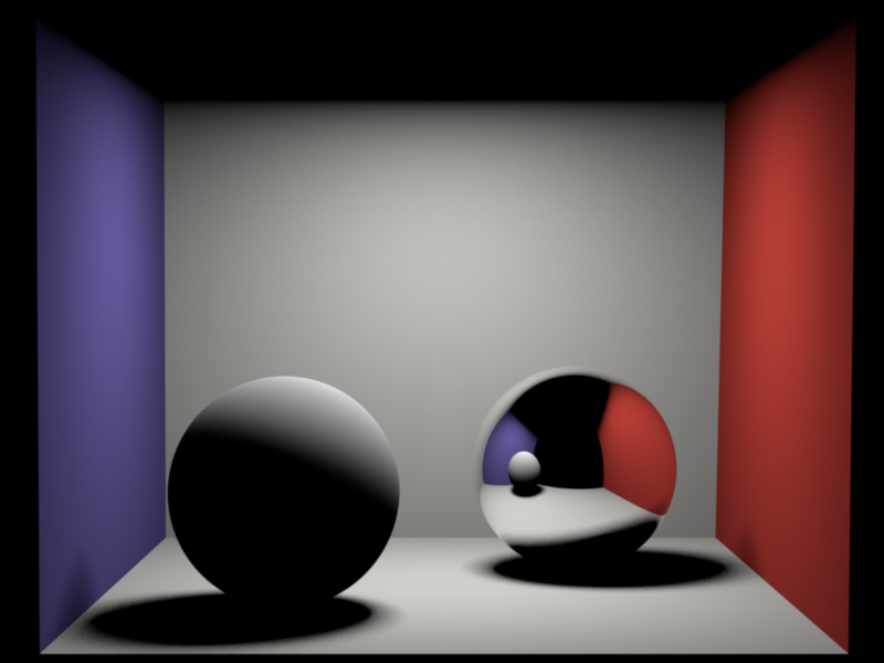
Render the scene scenes/pa2/cbox/cbox_whitted.xml and include a comparison against our reference solution: cbox_whitted.exr.

In this part we will extend the rudimentary interface in microfacet.cpp into a full-fledge reflectance model based on the microfacet theory. This process is split into four parts:

Part 1.1: Evaluating the Beckmann distribution

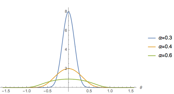
The Beckmann distribution models the probability density of normals on a random rough surface: \[ D(\theta, \phi) = \underbrace{\frac{1}{2\pi}}_{\text{azimuthal part}}\ \cdot\ \underbrace{\frac{2 e^{\frac{-\tan^2{\theta}}{\alpha^2}}}{\alpha^2 \cos^3 \theta}}_{\text{longitudinal part}}\!\!\!. \] The density includes an extra cosine factor for normalization purposes so that \[ \int_{0}^{2\pi}\int_0^{\frac{\pi}{2}} D(\theta, \phi)\sin\theta\,\mathrm{d}\theta\,\mathrm{d}\phi=1. \] Complete the function Warp::squareToBeckmannPdf in warp.cpp so that it evaluates \(D\) using the above definition. The function takes a normalized Cartesian 3D vector \(\omega\) as input, whose components can be interpreted using the following spherical coordinate representations: \[ \omega=\begin{pmatrix} \sin\theta\cos\phi\\ \sin\theta\sin\phi\\ \cos\theta \end{pmatrix} \] Take a look at the methods in the Frame class if you find yourself evaluating trigonometric functions in the body of Warp::squareToBeckmannPdf.

Part 1.2: Sampling the Beckmann distribution

Having implemented a way to query this distribution, we'll now want to generate points on the sphere that exactly follow the distribution. Note how the \(D(\theta,\phi)\) is symmetric around the north pole (in other words: its spherical coordinate representation is separable). Sampling can thus be split into two steps:

1. Uniformly sampling the azimuth \(\phi=2\pi\xi_1\) given a uniform variate \(\xi_1\).
   
   
2. Mapping a second uniform variate \(\xi_2\) through the inverse CDF of \(D\)'s longitudinal part to obtain \(\theta\).
   
   

Follow these two steps and implement the resulting sampling technique in Warp::squareToBeckmann. Try running the statistical test implemented in the warptest executable -- your implementation should pass the tests for different values of \(\alpha\). You do not need to include the test results in your report, this is just for your own guidance.

Part 1.3: Evaluating the Microfacet BRDF

The Microfacet BRDF in src/microfacet.cpp will be used to simulate platic-like materials. It consists of a linear blend between a diffuse BRDF (to simulate a potentially colored reflection from the interior of the material) and a rough dielectric microfacet BRDF (to simulate a non-colored specular reflection from the rough boundary). Implement Microfacet::eval() which evaluates the described microfacet BRDF for a given pair of directions in the local shading coordinate frame: \[ f_r(\bold{\omega_i},\bold{\omega_o}) = \frac{k_d}{\pi} + {k_s} \frac{D(\bold{\omega_{h}})~ F\left({(\bold{\omega_h} \cdot \bold{\omega_i})}, \eta_{e},\eta_{i}\right)~ G(\bold{\omega_i},\bold{\omega_o},\bold{\omega_{h}})}{4 \cos{\theta_i} \cos{\theta_o}\cos\theta_h}, ~~ \bold{\omega_{h}} = \frac{\bold{\omega_i} + \bold{\omega_o}}{\left|\left|\bold{\omega_i} + \bold{\omega_o}\right|\right|_2} \] Here, \(k_d \in [0,1]^3\) is the RGB diffuse reflection coefficient, \(k_s = 1 - \max(k_d)\), \(F\) is the Fresnel reflection coefficient (check common.cpp), \(\eta_e\) is the exterior index of refraction and \(\eta_i\) is the interior index of refraction. The various \(\cos\theta_k\) cosine factors relate to the angle that the corresponding direction \(\bold{\omega_k}\) makes with the Z axis in the local coordinate system. The shadowing term uses the rational function approximation: \[ G(\bold{\omega_i},\bold{\omega_o},\bold{\omega_{h}}) = G_1(\bold{\omega_i},\bold{\omega_{h}})~G_1(\bold{\omega_o},\bold{\omega_{h}}), \] \[ G_1(\bold{\omega_v},\bold{\omega_h}) = \chi^+\left(\frac{\bold{\omega_v}\cdot\bold{\omega_h}}{\bold{\omega_v}\cdot\bold{n}}\right) \begin{cases} \frac{3.535b+2.181b^2}{1+2.276b+2.577b^2}, & b \lt 1.6, \\ 1, & \text{otherwise}, \end{cases} \\ b = (\alpha \tan{\theta_v})^{-1}, ~~ \chi^+(c) = \begin{cases} 1, & c > 0, \\ 0, & c \le 0, \end{cases} \\ \] where \(\theta_v\) is the angle between the surface normal \(\bold{n}\) and the \(\omega_v\) argument of \(G_1\).

Part 1.4: Sampling the Microfacet BRDF

In this part you will generate samples according to the following density function: \[ k_s ~ D(\omega_h) ~ J_h + (1-k_s) \frac{\cos{\theta_o}}{\pi} \] where \(J_h = (4 (\omega_h \cdot \omega_o))^{-1}\) is the Jacobian of the half direction mapping. This an be done using the following sequence of steps:

1. Decide between a diffuse or a specular reflection by comparing a uniform variate \(\xi_1\) against \(k_s\)
2. Scale and potentially offset the uniform variate \(\xi_1\) so that it can be reused for a later sampling step
3. In the diffuse case, generate a cosine-weighted direction on the sphere following the approach in src/diffuse.cpp
4. In the specular case:
   1. Sample a normal from the Beckmann distribution using the approach from Part 1.2
   2. Reflect the incident direction using this normal to generate an outgoing direction.

Note that you will need to implement both Microfacet::sample() and Microfacet::pdf() to be able to run the following tests.

Validation

To obtain the full set of points for the previous exercises, you will need to validate the correctness of your code. The base code includes two XML files containing sequences of statistical tests that a correct implementation should be able to pass.

• scenes/pa2/tests/chi2test-microfacet.xml,
• scenes/pa2/tests/ttest-microfacet.xml

Next, use your whitted integrator from the previous assignment to render a microfacet Ajax bust and ensure that you can match our references:

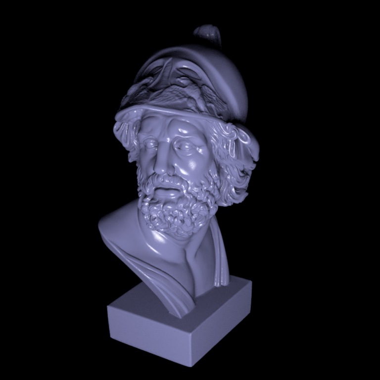
• scenes/pa2/ajax/ajax-rough.xml (reference: ajax-rough.exr)
• scenes/pa2/ajax/ajax-smooth.xml (reference: ajax-smooth.exr)

The warptestGUI also contains a \(\chi^2\) test for both the Beckmann distribution and the complete BRDF model, but this is just to facilitate debugging and visualization; the XML files are the real validation benchmark. Mention in your report if running these tests produces any errors.

In Part 1, you implemented a Whitted-style integrator that performed area light sampling on diffuse objects and BRDF sampling on specular objects. Now you'll extend this approach into a full path tracer that accounts for indirect illumination as well. We'll begin with a "simple" path tracer named src/path_simple.cpp that does not (yet) use multiple importance sampling. Part 4 involves adding MIS to create a full-featured path tracer that combines both sampling strategies to reduce variance.

This simple path tracer differs from src/whitted.cpp in the following ways:

1. When the camera ray hits a light source, the value returned by Li() should include the emitted radiance to account for directly visible light sources.
2. Instead of sampling a position on the light source or the BRDF, both are now done in each iteration. The direction sampled from the BRDF is used to estimate the indirect illumination component. This could be implemented using recursion, or more efficiently using a loop.

Use your implementation to render

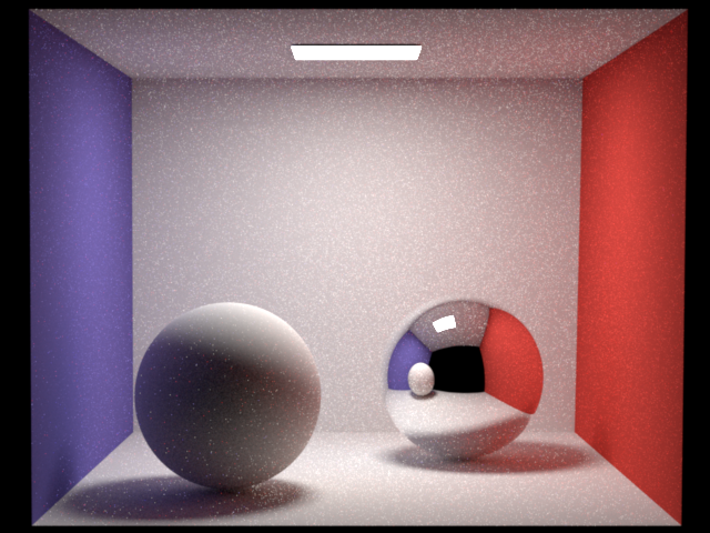
1. The Cornell box in scenes/pa2/cbox/cbox_simple.xml (reference: cbox_simple.exr).
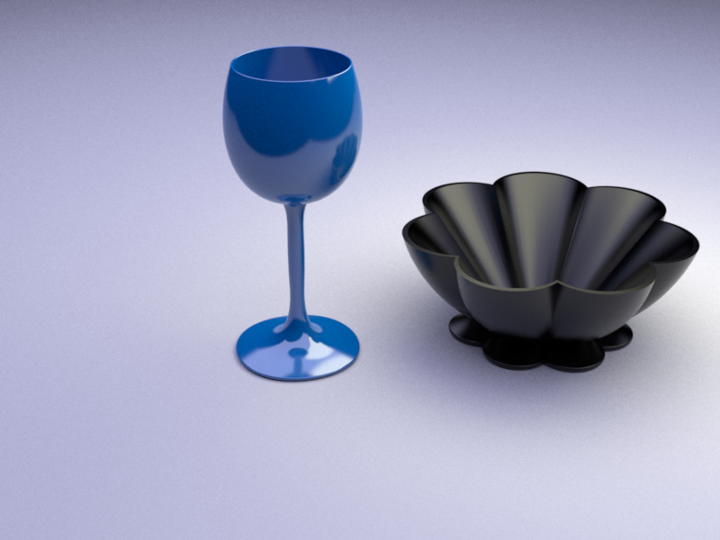
2. The Veach material test scene in scenes/pa2/veach_mi/veach_path_simple.xml (reference: veach_path_simple.exr).
3. The table test scene in scenes/pa2/table/table_path_simple.xml (reference: table_path_simple.exr).

The first scene only uses diffuse and specular materials and can be used to test your path tracer if you didn't do Part 2 of this assignment yet. The latter two assume that the microfacet model BRDF is ready.

Following Part 3, extend your path tracer with multiple importance sampling (MIS). This specifically entails:

1. When generating a sample on a light source, determine the density of this sampling strategy. Also compute the density (using BSDF::pdf()) with which the BRDF sampling strategy would hypothetically have sampled the same direction.
2. Weight the contribution of the light source sample using the following formula known as the balance heuristic: \[ w_\mathrm{Light}(p_\mathrm{Light}, p_\mathrm{BRDF}) = \frac{p_\mathrm{Light}}{p_\mathrm{Light} + p_\mathrm{BRDF}}. \] Remember that this only makes sense if both probabilities are expressed in the same measure (i.e. with respect to solid angles or unit area). This means that you will have convert one of them to the measure of the other (which one doesn't matter).
3. When generating a BRDF sample (which would normally only be used to estimate the indirect illumination component), check if it hits a light source. In this case, also use this sample to estimate the direct illumination component at the current vertex.
4. Once more, estimate the probability with which light source sampling would hypothetically have sampled this point, and weight the contribution of the sample using the balance heuristic: \[ w_\mathrm{BRDF}(p_\mathrm{Light}, p_\mathrm{BRDF}) = \frac{p_\mathrm{BRDF}}{p_\mathrm{Light} + p_\mathrm{BRDF}}. \] Note the changed numerator in the above expression.

Use your implementation to render

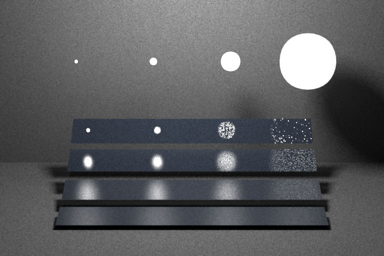
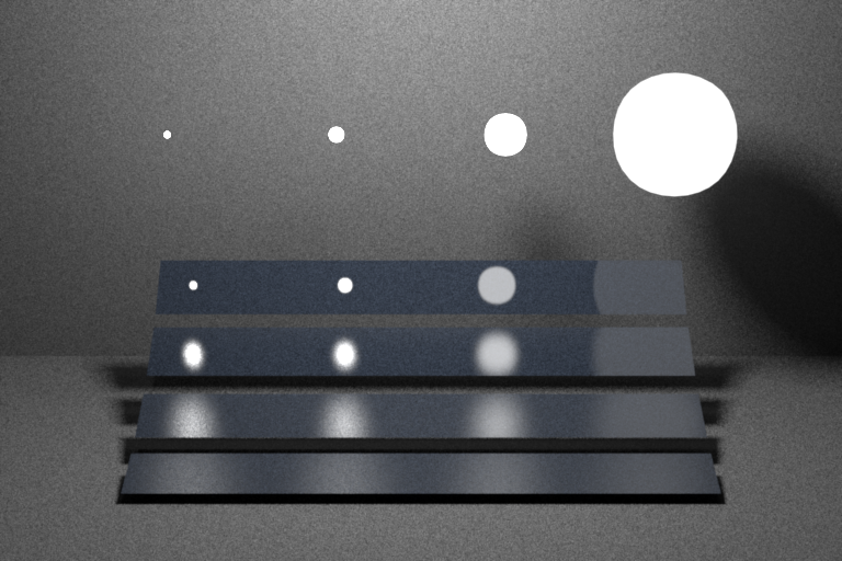
1. The Veach material test scene in scenes/pa2/veach_mi/veach_path.xml (reference: veach_path.exr).
2. The table test scene in scenes/pa2/table/table_path.xml (reference: table_path.exr).