ICS 180A, Spring 1997:
Strategy and board game programming

Lecture notes for April 22, 1997
Alpha-Beta Search

Shallow Pruning

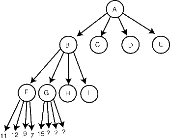
You've searched F, and found its children's evaluations to be 11, 12, 7, and 9; at this level of search, the first player is to move, and we expect him to choose the best of these values, 12. So, the minimax value of F is 12.

Now, you start searching G, and its first child returns a value of 15. When this happens, you know because of it that G's value will be at least 15, possibly even higher (if another of the children of G is even better). What this implies is that we don't expect the second player to move to G; from the second player's point of view, F's value of 12 is always better than G's value of 15 or higher. So, we know that G is not on the principal variation. We can prune the remaining children of G, not evaluate them, and return immediately from searching G, since any further work evaluating descendants of G would just be wasted.

In general, we can prune like we did in node G when one of its children returns a value better (from the point of view of the player whose turn it is at node G) than the previously computed evaluation of one of G's siblings.

Deep Pruning

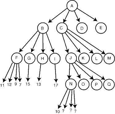
Other more complicated forms of pruning are possible as well. For example, suppose in the same search tree that we've evaluated all of G, H, and I to be better than 12, so that 12 is the total evaluation at node B. Now, we search node C, and two levels down, see an evaluation of 10 at node N:

We can use a more complicated line of reasoning to prune again. We know that N will return a 10 or smaller (the second player is to move, and wants to choose small numbers). We don't know whether this value of 10 or smaller will be returned at J as well, or whether one of the other children of J will be better. If a value 10 or smaller is returned from J to C, we can prune at C because it has a better sibling (B). So, in this case, further exploration of the children of N is pointless. The other case is that some other child of J returns a better value than 10; but again, in this case, further exploration of N is pointless. So as soon as we see 10, we can safely return from N.

Alpha-Beta Pseudocode

In general, when a returned value is better than the value of a sibling an even number of levels up in the tree, we can return immediately. If we pass the minimum value of any of these siblings in as a parameter beta to the search, we can do this pruning very efficiently. We also use another parameter alpha to keep track of the siblings at odd levels of the tree. Pruning using these two values is very simple; code to do so is listed below. Like last time, we use the negamax formulation, in which evaluations at alternate levels of the trees are negated.

double alphabeta(int depth, double alpha, double beta)
{
    if (depth <= 0 || game is over) return evaluation();
    generate and sort list of moves available in the position
    for (each move m) {
        make move m;
        double val = -alphabeta(depth - 1, -beta, -alpha);
        unmake move m;
        if (val >= beta) return val;
        if (val > alpha) alpha = val;
    }
    return alpha;
}

Aspiration Search

Alpha and beta define an interval of the real number line (alpha,beta) of the evaluations we consider interesting. If a value is greater than beta we prune and immediately return, because we know it's not part of the principal variation; we don't really care about the exact value, only that it's greater than beta. If a value is less than alpha, we don't prune, but we still don't consider it interesting, because we know there's a better move somewhere else in the tree.

But at the root of the tree, we don't know what range of evaluation values are likely to be interesting, and if we want to be sure of not accidentally pruning something important, we have to just set alpha=-infinity and beta=infinity.

However, especially if we are using iterated deepening, it is likely that we have a pretty good idea what the principal variation is going to look like. Suppose we guess that its value is going to be x (e.g., just let x be the value found when you previously searched to depth D-1), and let epsilon be a small number representing the amount by which we expect a depth-D search to vary from a depth-(D-1) search. We can then try calling alphabeta(D, x-epsilon, x+epsilon). Three different things can happen as a result:

1. The search might return a value within the interval (x-epsilon, x+epsilon). In this case, we know that it returned the correct value, and we can safely choose the move in the search tree leading to a node with that value.
2. The search might return a value v > x+epsilon. In this case, we know that the true search value is also > x+epsilon, but we don't know what it is (the correct principal variation might have been pruned as soon as we saw some other move having a value greater than beta). We have to adjust our guess x to be a higher value and try again (probably also with a larger value of epsilon). This condition is known as a fail high.
3. The search might return a value v < x-epsilon. In this case, we know that the true search value is also < x-epsilon, but we don't know what it is. We have to adjust our guess x to be a smaller value and try again (probably also with a larger value of epsilon). This condition is known as a fail low.

Analysis

In the best case, each node at depth D-1 will only examine one child at depth D before pruning, except that one node on the principal variation will not prune (if it did, the overall algorithm will end up failing high or failing low, which would certainly not be the best case).

At depth D-2, however, nobody can prune, because all the children returned values greater than or equal to the values of beta they were passed, which at depth D-2 are negated and become less than or equal to alpha.

Continuing up the tree, at depth D-3 everyone (except on the principal variation) prunes, and at depth D-4 nobody prunes, etc.

So, if the branching factor of the tree is B, the number of nodes increases by a factor of B at half the levels of tree, and stays pretty much constant (ignoring the principal variation) at the other half of the levels. So the total size of the part of the tree that gets searched ends up being roughly B^D/2 = sqrt(B)^D. Effectively, alpha-beta search ends up reducing the branching factor to the square root of its original value, and lets one search twice as deeply. For this reason it is an essential part of any minimax-based game-playing program.