7. Van der Waals Potential Energy

The pairwise potential energy, V(r) , between two non-bonded atoms can be expressed as a function of internuclear separation, r , as follows,

Graphically, if reqm is the equilibrium internuclear separation , and e is the well depth at reqm, then:

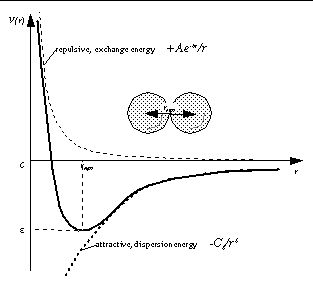
The exponential, repulsive, exchange energy is often approximated thus,

Hence pairwise-atomic interaction energies can be approximated using the following general equation,

where m and n are integers, and C n and C m are constants whose values depend on the depth of the energy well and the equilibrium separation of the two atoms' nuclei. Typically the 12-6 Lennard-Jones parameters ( n =12, m =6) are used to model the Van der Waals' forces 1 experienced between two instantaneous dipoles. However, the 12-10 form of this expression ( n =12, m =10) can be used to model hydrogen bonds (see "Modeling Hydrogen Bonds" below). Appendix See Parameters from AutoDock Version 1 gives the parameters which were distributed with the first (FORTRAN-77) version of AutoDock , and which have been used in numerous published articles.

A revised set of parameters has been calculated, which use the same Van der Waals radius of a given atom for all pairwise distances, no matter what the other atom. Likewise, the well-depths are consistently related. Let reqm, XX be the equilibrium separation between the nuclei of two like atoms, X, and let eXX be their pairwise potential energy or well depth. The combining rules for the Van der Waals radius, reqm, and the well depth, e, for two different atoms X and Y, are:
A derivation for the Lennard-Jones potential sometimes seen in text books invokes the parameter, s, thus,
Then the Lennard-Jones 12-6 potential becomes:
Hence, the coefficients C 12 and C 6 are given by:

We can derive a general relationship between the coefficients, equilibrium separation and well depth as follows. At the equilibrium separation, reqm, the potential energy is a minimumand equal to the well depth: in other words, V (reqm) = -e. The derivative of the potential with respect to separation will be zero at the minimum potential:

therefore:
so:
Substituting C m into the original equation for V ( r ), then at equilibrium we obtain,
Rearranging :
Therefore, the coefficient C n can be expressed in terms of n , m , e and reqm thus:
and, substituting into original equation for V ( r ),
In summary, then, we obtain the general equation for any n , m :

One final point worth making here is the effect of the ` smooth 0.500 ' command on the pairwise potentials. This is set in the AutoGrid input file (also known as the `GPF'). This is best illustrated with a diagram; note that this has the effect of widening the region of maximum affinity at e , and also reduces the potential energy at r=0 to a finite value:

Example reqm and e parameters for various AMBER atom types of carbon are shown in Table See AMBER parameters for carbon atom types. .

Using the equations describing C 12 and C 6 above, the following new set of 12-6 parameters were calculated shown in Table See Self-consistent Lennard-Jones 12-6 parameters, before multiplication by the free energy model coefficients. . These parameters may be used with AutoDock version 3.0, or alternatively, you may use or derive your own. Remember the linear regression coefficients for the van der Waals term has not been applied to the parameters in this table.

The above parameters yield the following graphs, for C, N, O and H atom types; the curves in order of increasing well-depth are: HH << CH < NH < OH << CC < CN < CO < NN < NO < OO:-

Grid maps are required only for those atom types present in the ligand being docked. For example, if the ligand being docked is a hydrocarbon, then only carbon and hydrogen grid maps would be required. In practice, however, non-polar hydrogens would not be modeled explicitly, so just the carbon grid map would be needed, for `united atom' carbons. This saves both disk space and computational time.