ICS 180A, Spring 1997:
Strategy and board game programming

Lecture notes for April 17, 1997
Minimax and negamax search

Game Trees

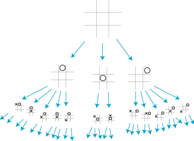
For any game, we can define a rooted tree (the "game tree") in which the nodes correspond to game positions, and the children of a node are the positions that can be reached from it in one move. For instance tic-tac-toe:

(Actually, the root of this tree should have nine children, but I've left out some symmetric cases. If the same board configuration arises from two different sequences of moves, we create two separate nodes, so this really is a tree. We'll see later when we talk about hashing how to take advantage of duplicated nodes to speed up the search -- we only need to search one copy of a position, and use the same search results everywhere else that position appears in the tree. We also assume that the players take turns moving, with no multiple moves or skipped turns; these complications can be dealt with by treating an entire sequence of actions by a single player as forming a single move. Finally, we'll assume this tree is finite, so that we're not dealing with a game that can go on forever or has infinitely many choices for a single move.)

There are three kinds of nodes in the tree:

1. Internal nodes at even levels correspond to positions in which the first player is to move.
2. Internal nodes at odd levels correspond to positions in which the second player is to move.
3. Leaves correspond to positions at which the game has ended. One player or the other has won, or perhaps the game is drawn.

Game Tree Evaluation

Suppose we have an internal node for which all children are leaves, so that the game is certain to end in one more move. Then we can assume that the player to move is going to pick the best move. If there is a leaf giving a won position for him, he will move to it and win. If not, but some leaf gives a drawn position for him, he will move to it and draw. But, if all leaves give won positions for his opponent, he will lose no matter what happens.

So, we know what the game outcome should be from nodes one level above the leaves. Once we know that, we can apply the same analysis bottom up, to determine the correct outcome from nodes two levels above the leaves, three levels up, and so on, until we reach the root of the tree. At each node, the position is won for the player on move if he can find a child of that node giving him a won position; it is drawn if he can find a child giving him a draw; and if neither of these holds then it is lost. This gives us an algorithm for playing games perfectly if only we had enough computation time, but for any reasonable game we won't have enough computation time. The trees are too big.

This also tells thus that a "correct" evaluation function needs to only have three values, win lose and draw. The evaluations we use in computer game programs have a wider range of real-number values only because they're inaccurate. If we represent a first-player win as the value +1, a draw as the value 0, and a second-player win as the value -1, then the value of each internal node in the game tree is the maximum or minimum of its children's values, depending on whether the first or second player is to move respectively.

Partial Game Trees

If both players really play this way, then we can determine the value of the leaf they will reach by the same min-max procedure outlined above: compute the value of each internal node as either the maximum or minimum of its children's values, depending on whether the first or second player is to move respectively. The path to this leaf is known as the principal variation. The basic principle of minimax game search is to expand a partial game tree, find the principal variation, and make the move forming the first step in this variation.

Breadth First and Depth First Search; Negamax Code

It's convenient to modify the game tree values slightly, so that we only need maximization operations rather than having to alternate between minima and maxima. At odd levels of the tree (nodes in which the second player is to move), negate the values defined above. Then at each node, these modified values can be found by computing the maximum of the negations of the node's children's values. Maybe this will make more sense if I write down some source code for game tree search:

// search game tree to given depth, return evaluation of root node
double negamax(int depth)
{
    if (depth <= 0 || game is over) return eval(pos);
    else {
        double e = -infty;
        for (each move m available in pos) {
            make move m;
            e = max(e, -negamax(depth - 1));
            unmake move m;
        }
        return e;
    }
}

// search game tree to given depth, return evaluation of root node
move rootsearch(int depth)
{
    double e = -infty;
    move mm;
    for (each move m available in pos) {
        make move m;
        double em = -negamax(depth - 1);
        if (e < em) {
            e = em;
            mm = m;
        }
        unmake move m;
    }
    return mm;
}

Analysis of negamax: branching factor, depth

With these assumptions, it's easy to write down a formula for the amount of time the negamax program uses: it's just proportional to the number of tree nodes expanded. (It may look like we should multiply by something since there is a loop nested within each call to negamax, but the time spent in this loop can be charged to the recursive calls made in it.) If the branching factor is b and the depth is d, this number is

The stuff in parentheses at the end of the formula is very close to one, so the overall time is very close to b^d.

If our game doesn't meet the strict assumptions above, we can work backwards and define the effective branching factor to be whatever value of b works to make the formula above describe our program's running time. Even less formally, we'll use "branching factor" to describe the average number of moves available from a "typical" position in a game.

What can we say about this formula? First, it's exponential. This means that we won't be able to search too many nodes; if we get a computer twice as fast as the old one, we will only be able to increase d by some small number of levels. Second, it depends very strongly on the branching factor b. In a game with a small branching factor (like checkers, in which there may often be as few as three moves to search) we can search much deeper than chess (which may have 30 or so moves in a position) or go (hundreds of moves in a position). So we'd like b to be as small as possible, but unfortunately it's more a function of what game we're working on and less a function of how well we can program. However, the technique I'll talk about next time, alpha-beta pruning, acts to reduce the effective branching factor considerably: if we're lucky, to the square root of its value in unpruned game trees, which lets us search to twice the depth we might without using alpha-beta.

Iterated Deepening

depth = 0
while (enough time left for another level of search) {
    depth++;
    m = rootsearch(depth);
}
make move m